Data collection modes

ROCm Systems Profiler supports several modes of recording trace and profiling data for your application.

Note

For an explanation of the terms used in this topic, see the ROCm Systems Profiler glossary.

Mode	Description
Binary Instrumentation	Locates functions (and loops, if desired) in the binary and inserts snippets at the entry and exit
Statistical Sampling	Periodically pauses application at specified intervals and records various metrics for the given call stack
Callback APIs	Parallelism frameworks such as ROCm, OpenMP, and Kokkos make callbacks into ROCm Systems Profiler to provide information about the work the API is performing
Dynamic Symbol Interception	Wrap function symbols defined in a position independent dynamic library/executable, like pthread_mutex_lock in libpthread.so or MPI_Init in the MPI library
User API	User-defined regions and controls for User API ROCm Systems Profiler

The two most generic and important modes are binary instrumentation and statistical sampling. It is important to understand their advantages and disadvantages. Binary instrumentation and statistical sampling can be performed with the rocprof-sys-instrument executable. For statistical sampling, it’s highly recommended to use the rocprof-sys-sample executable instead if binary instrumentation isn’t required or needed. Callback APIs and dynamic symbol interception can be utilized with either tool.

Binary instrumentation

Binary instrumentation lets you record deterministic measurements for every single invocation of a given function. Binary instrumentation effectively adds instructions to the target application to collect the required information. It therefore has the potential to cause performance changes which might, in some cases, lead to inaccurate results. The effect depends on the information being collected and which features are activated in ROCm Systems Profiler. For example, collecting only the wall-clock timing data has less of an effect than collecting the wall-clock timing, CPU-clock timing, memory usage, cache-misses, and number of instructions that were run. Similarly, collecting a flat profile has less overhead than a hierarchical profile and collecting a trace OR a profile has less overhead than collecting a trace AND a profile.

In ROCm Systems Profiler, the primary heuristic for controlling the overhead with binary instrumentation is the minimum number of instructions for selecting functions for instrumentation.

Statistical sampling

Statistical call-stack sampling periodically interrupts the application at regular intervals using operating system interrupts. Sampling is typically less numerically accurate and specific, but the target program runs at nearly full speed. In contrast to the data derived from binary instrumentation, the resulting data is not exact but is instead a statistical approximation. However, sampling often provides a more accurate picture of the application execution because it is less intrusive to the target application and has fewer side effects on memory caches or instruction decoding pipelines. Furthermore, because sampling does not affect the execution speed as much, is it relatively immune to over-evaluating the cost of small, frequently called functions or “tight” loops.

In ROCm Systems Profiler, the overhead for statistical sampling depends on the sampling rate and whether the samples are taken with respect to the CPU time and/or real time.

Binary instrumentation vs. statistical sampling example

Consider the following code:

long fib(long n)
{
     if(n < 2) return n;
     return fib(n - 1) + fib(n - 2);
}

void run(long n)
{
     long result = fib(n);
     printf("[%li] fibonacci(%li) = %li\n", i, n, result);
}

int main(int argc, char** argv)
{
     long nfib = 30;
     long nitr = 10;
     if(argc > 1) nfib = atol(argv[1]);
     if(argc > 2) nitr = atol(argv[2]);

     for(long i = 0; i < nitr; ++i)
         run(nfib);

     return 0;
}

Binary instrumentation of the fib function will record every single invocation of the function. For a very small function such as fib, this results in significant overhead since this simple function takes about 20 instructions, whereas the entry and exit snippets are ~1024 instructions. Therefore, you generally want to avoid instrumenting functions where the instrumented function has significantly fewer instructions than entry and exit instrumentation. (Note that many of the instructions in entry and exit functions are either logging functions or depend on the runtime settings and thus might never run). However, due to the number of potential instructions in the entry and exit snippets, the default behavior of rocprof-sys-instrument is to only instrument functions which contain at least 1024 instructions.

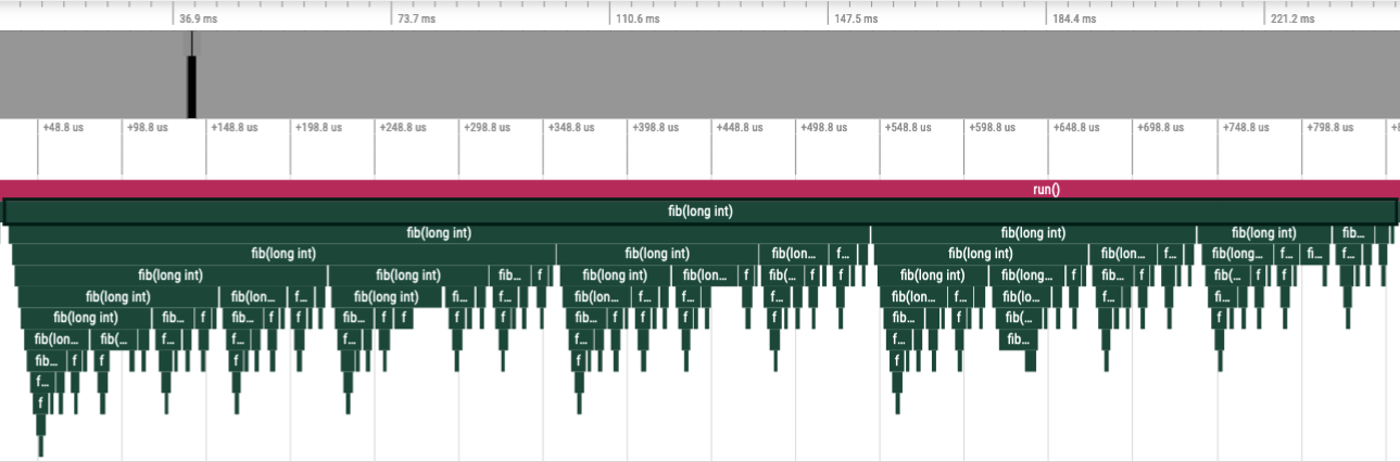
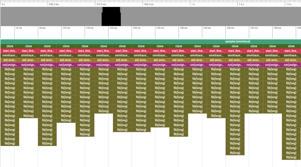
However, recording every single invocation of the function can be extremely useful for detecting anomalies, such as profiles that show minimum or maximum values much smaller or larger than the average or a high standard deviation. In this case, the traces help you identify exactly when and where those instances deviated from the norm. Compare the level of detail in the following traces. In the top image, every instance of the fib function is instrumented, while in the bottom image, the fib call-stack is derived via sampling.

Binary instrumentation of the Fibonacci function

Statistical sampling of the Fibonacci function

Overview of profiling modes

ROCm Systems Profiler provides several complementary profiling approaches that can be used independently or in combination. Profiling modes are controlled via the ROCPROFSYS_MODE environment variable, which determines the active backends and features.

Available values for ROCPROFSYS_MODE: trace, sampling, causal, and coverage.

Primary collection modes

Mode	Purpose
Trace mode	Event tracing
Profile mode	High-level summary profiles
Sampling mode	Statistical call-stack sampling
Causal mode	Performance impact analysis
Coverage mode	Code coverage analysis

Trace mode (default)

Tracing mode generates comprehensive, deterministic traces of every event and measurement during application execution. This mode can be enabled using ROCPROFSYS_TRACE=true, ROCPROFSYS_MODE=trace, or by using the --trace / -T CLI flag.

ROCm Systems Profiler provides two tracing implementations:

• Cached Mode (default): By default, when tracing is enabled, ROCm Systems Profiler uses deferred trace generation with minimal runtime overhead. Trace data is buffered during execution and written after the application completes, significantly reducing performance impact during profiling.

• Legacy Mode: ROCPROFSYS_TRACE_LEGACY=true or --trace-legacy / -L enables direct mode where trace data is written immediately during execution. This mode provides real-time trace generation but has higher runtime overhead compared to cached mode.

Additional configuration options to control the tracing behavior include:

• ROCPROFSYS_TRACE_DELAY (--trace-wait): Delay before starting trace collection (in seconds).

• ROCPROFSYS_TRACE_DURATION (--trace-duration): Duration of trace collection (in seconds).

• ROCPROFSYS_TRACE_PERIODS (--trace-periods): Specifies multiple delay/duration periods in the format <DELAY>:<DURATION>, <DELAY>:<DURATION>:<REPEAT>, or <DELAY>:<DURATION>:<REPEAT>:<CLOCK_ID>.

• ROCPROFSYS_TRACE_PERIOD_CLOCK_ID (--trace-clock-id): Clock type for timing, such as realtime, monotonic, cputime.

Profile mode

Profile mode generates high-level summary profiles with statistical aggregations (mean, min, max, stddev). This mode can be enabled using ROCPROFSYS_PROFILE=true. This mode uses the Timemory backend. When tracing is enabled, profiling is turned off by default, and vice versa. However, both modes can be turned on at the same time.

By default, only wall-clock timing is collected. Additional metrics can be configured using ROCPROFSYS_TIMEMORY_COMPONENTS, which enables hardware counters (via PAPI), CPU, memory, and system metrics. To view the available components, use: rocprof-sys-avail --components --description.

Profile types:

• Flat Profile (--flat-profile): Aggregated metrics per function across all contexts.

• Hierarchical Profile (--profile): Metrics organized by call-stack context.

Tip

Start with a flat profile to identify high-impact functions, then use a hierarchical profile to analyze critical paths.

Sampling mode

Sampling uses statistical call-stack sampling through periodic software interrupts per thread, as described in Sampling the call stack.

Sampling types:

1. CPU-Time sampling (default)

• Enabled using ROCPROFSYS_SAMPLING_CPUTIME=ON or --cputime (rocprof-sys-sample), --sample-cputime (rocprof-sys-run). The sampling can be controlled using:

  • ROCPROFSYS_SAMPLING_CPUTIME_FREQ

  • ROCPROFSYS_SAMPLING_CPUTIME_DELAY

  • ROCPROFSYS_SAMPLING_CPUTIME_SIGNAL

2. Real-Time sampling

• Enabled using ROCPROFSYS_SAMPLING_REALTIME=ON or --realtime (rocprof-sys-sample), --sample-realtime (rocprof-sys-run). The sampling can be controlled using:

  • ROCPROFSYS_SAMPLING_REALTIME_FREQ

  • ROCPROFSYS_SAMPLING_REALTIME_DELAY

  • ROCPROFSYS_SAMPLING_REALTIME_SIGNAL

3. Overflow sampling

• Enabled using ROCPROFSYS_SAMPLING_OVERFLOW=ON or --sample-overflow (rocprof-sys-run). It requires Linux perf support (/proc/sys/kernel/perf_event_paranoid <= 2) as described in ROCPROFSYS_PAPI_EVENTS. The sampling can be controlled using:

  • ROCPROFSYS_SAMPLING_OVERFLOW_FREQ

  • ROCPROFSYS_SAMPLING_OVERFLOW_EVENT

  • ROCPROFSYS_SAMPLING_OVERFLOW_SIGNAL

  • ROCPROFSYS_SAMPLING_OVERFLOW_TIDS

4. Process sampling

• Enabled using ROCPROFSYS_USE_PROCESS_SAMPLING=ON (default ON). The sampling can be controlled using:

  • ROCPROFSYS_PROCESS_SAMPLING_FREQ

  • ROCPROFSYS_SAMPLING_CPUS

  • ROCPROFSYS_SAMPLING_GPUS

Note

If sampling is enabled but no specific type is selected, CPU-time sampling is used by default.

To enable sampling:

1. Use rocprof-sys-sample (auto-enables sampling).

2. Set ROCPROFSYS_USE_SAMPLING=ON and ROCPROFSYS_MODE=sampling.

3. Use -S or --sample with rocprof-sys-run.

4. Use -M sampling or --mode sampling with rocprof-sys-instrument. Use of rocprof-sys-sample is recommended over rocprof-sys-instrument -M sampling when binary instrumentation is not necessary. For more details, see Sampling the call stack.

Causal mode

Causal profiling quantifies the potential impact of optimizations in parallel code and predicts where efforts should be focused as described in Performing causal profiling. This mode can be enabled using: ROCPROFSYS_USE_CAUSAL=true or ROCPROFSYS_MODE=causal.

Coverage mode

Coverage mode tracks which parts of your code are executed during a run. It uses binary instrumentation to record function and/or basic block execution. This mode can be enabled using: rocprof-sys-instrument -M coverage.

Granularity options:

• Function-level: --coverage=function (CODECOV_FUNCTION)

• Basic block-level: --coverage=basic_block (CODECOV_BASIC_BLOCK)

Note

Coverage mode disables several other features and all other modes to reduce overhead.