Profiling Llama-4 inference with vLLM#
Authors: Shekhar Pandey and Liz Li
Knowledge level: Intermediate
Profiling is essential for understanding the performance bottlenecks in large language model inference pipelines. This tutorial walks you through the process of profiling the Llama-4 Scout-17B-16E-Instruct model using the vLLM framework on AMD GPUs with ROCm. You’ll capture detailed kernel traces and later visualize them using Perfetto.
Prerequisites#
Before starting this tutorial, ensure you have the following:
Access to the gated Llama-4 Scout-17B-16E-Instruct model
Access to Perfetto UI
Hardware#
AMD GPUs: Ensure you are using an AMD GPU, such as the Instinct™ MI300X or Radeon Pro W7900, with ROCm support and that your system meets the official requirements.
Software#
ROCm 6.3, 6.4: Install and verify ROCm by following the ROCm install guide. Verify your ROCm installation by running this command:
amd-smi
This command lists your AMD GPUs with relevant details.
Note: For ROCm 6.4 and earlier, use the
rocm-smicommand instead.Docker: Ensure Docker is installed and configured correctly. See the Docker installation guide for more information.
Prepare the training environment#
Follow these steps to configure your tutorial environment:
1. Pull the Docker image#
Ensure your system meets the system requirements.
Pull the Docker image required for this tutorial:
docker pull rocm/vllm-dev:main
2. Launch the Docker container#
Launch the Docker container in a terminal on your server and map the necessary directories.
docker run -it --rm \
  --network=host \
  --device=/dev/kfd \
  --device=/dev/dri \
  --group-add=video \
  --ipc=host \
  --cap-add=SYS_PTRACE \
  --security-opt seccomp=unconfined \
  --shm-size 8G \
  -v $(pwd):/workspace \
  -w /workspace/notebooks \
  rocm/vllm:latest
Note: This command mounts the current directory to the /workspace directory in the container. Ensure the notebook file is either copied to this directory before running the Docker command or uploaded into the Jupyter Notebook environment after it starts. Save the token or URL provided in the terminal output to access the notebook from your web browser. You can download this notebook from the AI Developer Hub GitHub repository.
3. Install and launch Jupyter#
Inside the Docker container, install Jupyter using the following command:
pip install jupyter
Start the Jupyter server:
jupyter-lab --ip=0.0.0.0 --port=8888 --no-browser --allow-root
Step-by-step process#
Follow these steps to profile the Llama-4 model and capture the kernel traces.
Step 1: Logging in to Hugging Face#
Provide your Hugging Face token
You’ll require a Hugging Face API token to access Llama-4. Generate your token at Hugging Face Tokens and request access for Llama-4-Scout 17B-16E-Instruct. Tokens typically start with “hf_”.
Run the following interactive block in your Jupyter notebook to set up the token:
Note: Uncheck the “Add token as Git credential” option.
from huggingface_hub import notebook_login, HfApi

# Prompt the user to log in
notebook_login()
Verify that your token was accepted correctly:
from huggingface_hub import HfApi

try:
    api = HfApi()
    user_info = api.whoami()
    print(f"Token validated successfully! Logged in as: {user_info['name']}")
except Exception as e:
    print(f"Token validation failed. Error: {e}")
Step 2: Start the vLLM server with a profiler configuration#
Open a new terminal tab inside your JupyterLab session. In this new terminal, run the following commands. Keep the terminal open.
mkdir -p /profile
export VLLM_TORCH_PROFILER_DIR=/profile

# Start the vLLM server with standard configs
RCCL_MSCCL_ENABLE=0 \
VLLM_USE_V1=1 \
VLLM_WORKER_MULTIPROC_METHOD=spawn \
VLLM_USE_MODELSCOPE=False \
VLLM_USE_TRITON_FLASH_ATTN=0 \
vllm serve meta-llama/Llama-4-Scout-17B-16E-Instruct \
    --disable-log-requests \
    -tp 8 \
    --max-num-seqs 64 \
    --no-enable-prefix-caching \
    --max_num_batched_tokens=320000 \
    --max-model-len 32000
Step 3: Run the benchmark and capture the trace#
With the server running, trigger a synthetic benchmark request to generate traffic and collect the profiling data:
!vllm bench serve \
    --model meta-llama/Llama-4-Scout-17B-16E-Instruct \
    --dataset-name random \
    --random-input-len 2000 \
    --random-output-len 10 \
    --max-concurrency 64 \
    --num-prompts 64 \
    --ignore-eos \
    --percentile_metrics ttft,tpot,itl,e2el \
    --profile
Ensure you add the --profile flag, which starts the profiler before the benchmark starts and then stops it afterwards and generates the trace.
NOTE: After the execution of the cell above completes, stop the vLLM server you started in the other terminal by pressing Ctrl-C.
Step 4 : Visualize the trace using Perfetto UI#
After the trace is generated, unzip it. The trace is saved in the JSON format. To visualize it, use Perfetto UI, a powerful trace viewer built for large-scale profiling data. This helps uncover latency bottlenecks, CPU–GPU overlap, and kernel-level inefficiencies in your inference pipeline. To visualize the trace, follow these steps:
Go to https://ui.perfetto.dev.
Click “Open trace file”.
Upload the
.jsonfile.
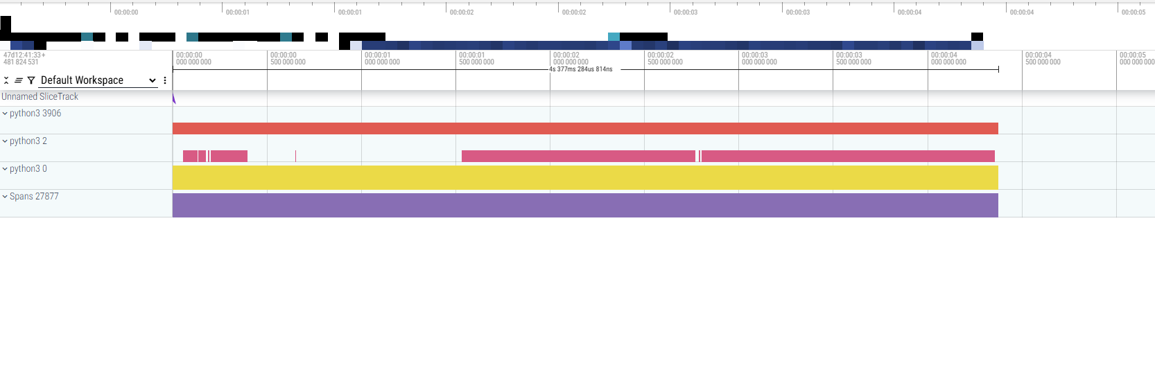
After you open the trace, it will look somewhat like this:
Understanding the prefill and decode timelines#
Now zoom into the trace to interpret what each slice reveals about the Llama-4 execution stages. Here’s a close-up of two important process timelines captured in Perfetto:
Note: The focus of this section is on the first two tracks: python3 3906 and python3 2.
python3 3906: Asynchronous CPU callsThe orange slice under
python3 3906shows the execution of high-level model code on the CPU. It includes:Calls like
execute_model,forward, andhipMemcpyWithStreamPyTorch internals such as
aten::toandaten::copy_The actual forward pass for
Llama4ForCausalLMand memory transfers
This slice reflects the CPU-side orchestration of inference, from input preparation to dispatching kernels to the GPU.
python3 2: GPU kernel timelineThe pink slice under
python3 2is where GPU kernel execution is visualized. This slice represents actual compute work being done by the GPU after the CPU enqueues the tasks.Here’s the key insight:
There is a clear gap between two bursts of kernel execution.
This gap separates two distinct phases:
Before the gap: This is the “prefill” stage, where the initial prompt is encoded, and attention and cache states are populated.
After the gap: This is the “decode” stage, where the model generates tokens, typically using cached key/value tensors.
Understanding kernel timelines#
When you expand the python3 2 timeline in Perfetto, you’ll see two distinct GPU streams representing different types of operations executed on the device:

Note: This zoomed-in view helps you distinguish between computation kernels and communication operations.
Stream
3 3: All GPU kernelsStream
3 3is the primary compute stream, where all GPU kernel executions are scheduled. This includes:MatMuland GEMM operationsFused MLP and attention blocks
Positional encodings and LayerNorms
Any fused or element-wise kernels
This stream is densely packed, showing the bulk of the model inference activities The rhythm and spacing of these kernels help diagnose things like:
Load balancing across tensor parallel ranks
Gaps between kernel launches
Prefill versus decode phases (based on the density before and after the gaps)
Stream
3 8: AllGather kernelsStream
3 8is used specifically for AllGather operations, which are part of the tensor parallel communication process. These kernels:Synchronize activations across devices in multi-GPU setups
Typically occur between layer boundaries
Are crucial in
tp=8setups for syncing partial outputs across eight shards
Step 5: Zoom in to analyze the attention forward kernel#
Attention is at the heart of all Transformer-based language models and Llama-4 is no exception. Profiling its attention forward kernel gives us critical insights into its computational efficiency. Dive into the trace to inspect it at the kernel level.
Zoom into the kernel timeline#
Navigate to
python3 2and then tostream 3 3in the Perfetto UI.Scroll with the mouse or drag to zoom into a cluster of dense kernels.
Hover over one of the prominent kernels. You should see a label like
_fwd_kernel.
Here’s an example image from the trace:
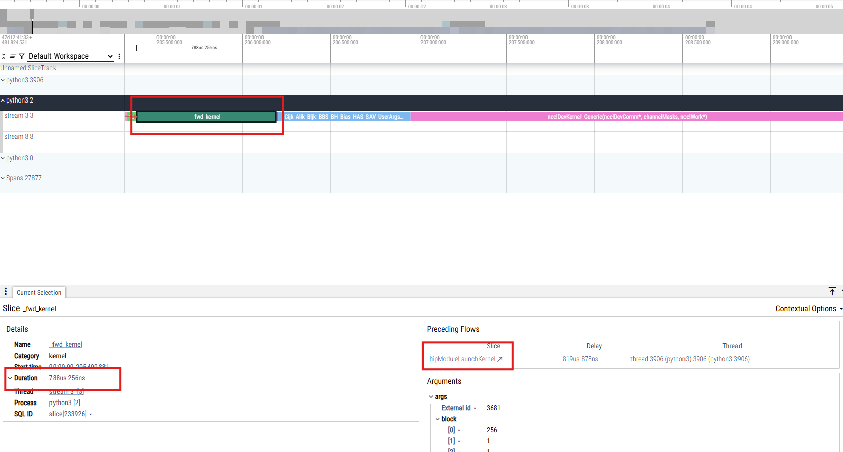
Understanding the kernel slice#
From the details panel below the trace view, you can extract the following:
Field |
Value |
|---|---|
Name |
|
Category |
|
Stream |
|
Process |
|
Duration |
|
Launch delay |
|
This kernel is part of the multi-head attention forward pass, one of the most compute-heavy operations in inference.
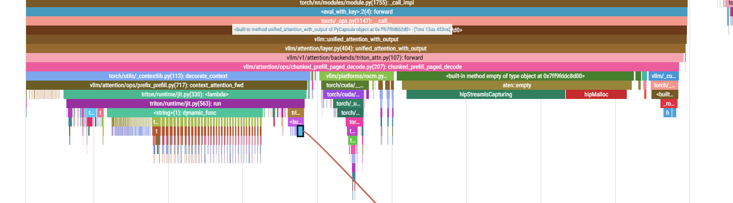
Tracing back to the CPU#
Inside the kernel details, near the preceding flows, you’ll find hipModuleLaunchKernel.
Click this to jump back to the CPU thread (python3 3906), shown in blue in the image below, which issued this kernel launch. This feature is incredibly useful for:
Mapping GPU operations to their Python or C++ call stack
Identifying bottlenecks in dispatch or synchronization
Understanding how long the CPU takes to enqueue work on the GPU
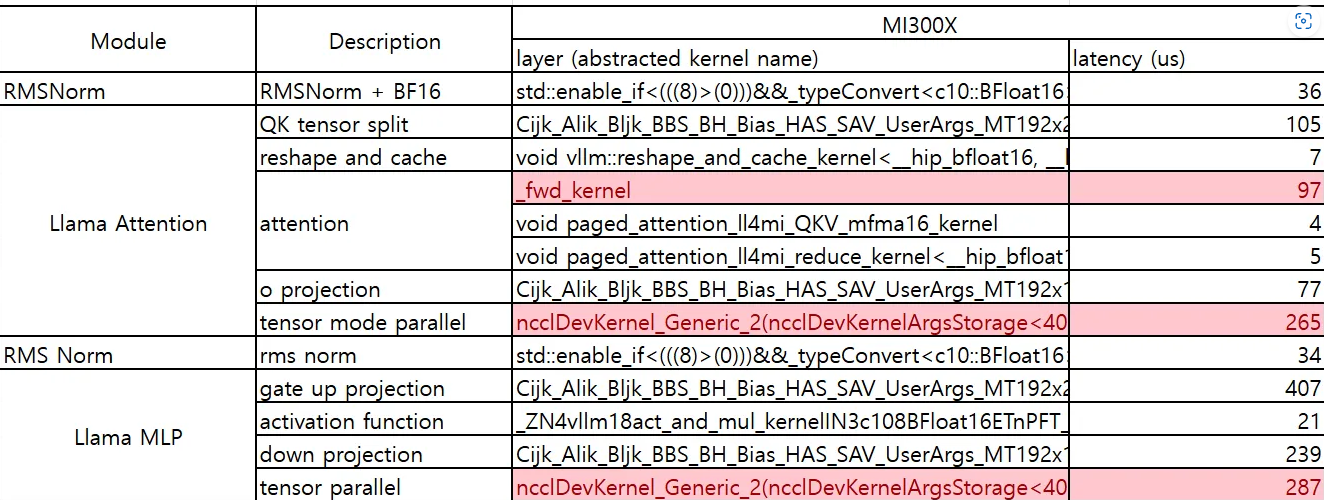
Following the process above, you can track how much time each kernel takes in both the prefill and decode stage. A short summary for one kernel is shown in the chart below.
Step 6: Programmatic analysis and extracting the GPU kernel timeline with Python#
To go beyond visual inspection, you can also parse the trace programmatically to list all GPU kernels and their durations. This is helpful when you’re tracking:
Kernel launch patterns
Duration spikes
Gaps or anomalies in execution
Here’s a minimal Python script that reads the trace.json file and lists all GPU kernels sorted by start time:
Decompress the .gz trace file into trace.json.
!gunzip -c /profile/$(ls /profile | head -n 1) > trace.json
Run the cell below, which lists all GPU kernels sorted by start time.
import json

# Load the trace
with open("trace.json", "r") as f:
    trace = json.load(f)

gpu_kernels = []

# Extract GPU kernel events
for event in trace["traceEvents"]:
    if event.get("ph") != "X":
        continue

    cat = event.get("cat", "").lower()
    name = event.get("name", "")
    start_time = event["ts"]
    duration = event.get("dur", 0)

    if "cuda" in cat or "kernel" in cat:
        gpu_kernels.append({
            "name": name,
            "start": start_time,
            "duration": duration
        })

# Print all GPU kernels with their durations
print(f"{'GPU Kernel':<60} {'Start (us)':<15} {'Duration (us)':<15}")
print("-" * 90)
for k in sorted(gpu_kernels, key=lambda x: x["start"]):
    print(f"{k['name']:<60} {k['start']:<15} {k['duration']:<15}")
Conclusion#
In this tutorial, you walked through the end-to-end process of profiling Llama-4 inference on AMD GPUs using vLLM, including:
Setting up the container with ROCm and vLLM
Enabling and capturing detailed performance traces
Visualizing CPU-GPU interactions with Perfetto
Zooming into kernel-level activity for attention blocks
Programmatically analyzing trace logs using Python