MLA decoding kernel of the AITER library to accelerate LLM inference#
Imagine you’re deploying a large language model such as DeepSeek-V3/R1 on AMD Instinct™ GPUs, when suddenly the Multi Latent Attention (MLA) in the decoding phase becomes a performance bottleneck. Token generation feels sluggish, and latency keeps accumulating, degrading the user experience. This is where the AMD AITER library comes to the rescue, dramatically accelerating the MLA decode attention kernel to breathe new life into your model.
AITER is a high-performance operator library from AMD, optimized for AI workloads on AMD Instinct GPUs. It’s indispensable when:
Operator performance falls far short of the theoretical potential.
Specific operators become inference bottlenecks.
You need architecture-specific optimizations for AMD Instinct GPUs.
This tutorial guides you step-by-step through integrating the AITER MLA decode attention kernel to supercharge LLM inference with AMD Instinct GPUs. This will greatly accelerate kernel performance, with different context lengths, compared to native PyTorch implementations. You’ll start by setting up the MLA decode attention kernel.
Tip: Kernels in the AITER library are already integrated into popular LLM inference frameworks such as vLLM and SGLang. This means you can also achieve significant performance gains from the AITER library on AMD Instinct GPUs through these frameworks!
Prerequisites: Setting up the acceleration environment#
This tutorial was developed and tested using the following setup, which is recommended to reproduce the same model acceleration with AMD Instinct GPUs.
Operating System#
Ubuntu 22.04: Ensure your system is running Ubuntu version 22.04.
Hardware#
AMD Instinct GPUs: Ensure you are using an AMD Instinct GPU with ROCm™ software support and that your system meets the official requirements.
Software#
ROCm 6.3.1: Install and verify ROCm by following the ROCm install guide.
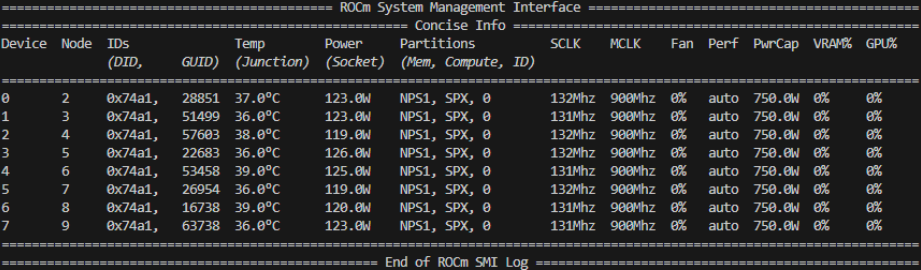
After installation, confirm your setup using the
rocm-smicommand.rocm-smi
This command lists the available AMD GPUs and their status:
Docker: For containerized deployment, ensure Docker is installed and configured correctly. Follow the Docker installation guide for your operating system.
Note: Ensure the Docker permissions are correctly configured. To configure permissions to allow non-root access, run the following commands:
sudo usermod -aG docker $USER
newgrp docker
Verify Docker is working correctly:
docker run hello-world
Quick start development environment set up#
This tutorial uses the prebuilt ROCm PyTorch image.
Step 1: Launch the ROCm PyTorch Docker container#
Launch the Docker container. This image is a turnkey solution with pre-configured dependencies:
docker run -it --rm \
  --network=host \
  --device=/dev/kfd \
  --device=/dev/dri \
  --group-add=video \
  --ipc=host \
  --cap-add=SYS_PTRACE \
  --security-opt seccomp=unconfined \
  --shm-size 8G \
  -v $(pwd):/workspace \
  -w /workspace \
  rocm/pytorch:latest
Note: This command mounts the current directory to the /workspace directory in the container for easy file access. It lets you perform all work in this Docker container, including manually installing AITER, and get started with the following hands-on, practical examples.
Step 2: Launch Jupyter Notebooks in the container#
Inside the Docker container, install JupyterLab using the following command:
pip install jupyter
Start the Jupyter server:
jupyter-lab --ip=0.0.0.0 --port=8888 --no-browser --allow-root
Note: If port 8888 is occupied, specify a different port, such as --port=8890. The rest of this tutorial can run as interactive blocks in your Jupyter notebook after you upload this tutorial to your server.
Step 3: Manually install the AITER library#
AITER is a rapidly expanding library with many powerful features. To install AITER, use these commands:
%%bash
git clone --recursive https://github.com/ROCm/aiter.git
cd aiter
python3 setup.py develop
export PYTHONPATH=$PYTHONPATH:/workspace/aiter
Note: If you’re running Jupyter and AITER in your environment, set PYTHONPATH accordingly.
Understanding the MLA decode attention kernel#
You can find the MLA decoding attention kernel definition in the AITER source code. It requires a minimum of eight input parameters and can accept three additional optional inputs. Here’s the function definition for mla_decode_fwd, including the parameters:
def mla_decode_fwd(
    q,                   # [batch_size, num_heads, kv_lora_rank + qk_rope_dim]
    kv_buffer,           # [num_pages, page_size, num_heads_kv, qk_head_dim]
    o,                   # Output buffer [batch_size, num_heads, kv_lora_rank]
    qo_indptr,           # Query sequence pointer [batch_size + 1]
    kv_indptr,           # KV sequence pointer [batch_size + 1]
    kv_indices,          # KV indices [kv_indptr[-1]]
    kv_last_page_lens,   # Last page sizes [batch_size]
    max_seqlen_q,        # Maximum query sequence length
    sm_scale=None,       # Scaling factor (default: 1.0/sqrt(qk_head_dim))
    logit_cap=0.0,       # (Under development)
    num_kv_splits=None,  # KV splits (auto-determined)
):
Each parameter has specific shape requirements, so proper configuration is key to optimal performance:
q (
torch.tensortype): This is the query tensor with shape requirements like[batch_size, num_heads, kv_lora_rank + qk_rope_dim].kv buffer (
torch.tensortype): This is the total kv cache tensor with shape requirements like[num_pages, page_size, num_heads_kv, qk_head_dim], wherenum_heads_kvis always1in the decode phase, andnum_pagesandpage_sizejointly represent the pageable kv cache. Whenpage_size = 1, the kv cache is set to the original representation, which wastes a lot of GPU memory.o (
torch.tensortype): This is the output buffer. Themla_decode_fwdfunction will place the result intoo, which has shape requirements like[batch_size, num_heads, kv_lora_rank].qo_indptr (
torch.tensortype): This is a pointer to the start address of each query and output sequence, with shape requirements like[batch_size + 1]. When the sequence length of each sequence in a batch is different, theqo_indptris used to record this information, which helps handle each sequence correctly.kv_indptr (
torch.tensortype): This is a pointer to the start address of each context/kv sequence, with shape requirements like[batch_size + 1]. Each query sequence is different within a batch, and the sequence of answers is also different, so the context/kv sequence lengths are also different. Thekv_indptrvariable records this information to help handle each context/kv of the query sequence correctly.kv_indices (
torch.tensortype): This contains the concrete kv start indices of each sequence. It has shape requirements like[kv_indptr[-1]].kv_last_page_lens (
torch.tensortype): This is the last page size of each sequence, with shape requirements like[batch_size].max_seqlen_q: (
torch.tensortype): This is the max sequence length across all the queries in this batch.sm_scale (
scalartype): This is equal to1.0 / (qk_head_dim**0.5), which represents the denominator in the scale dot product attention formula.logit_cap: This is a work in progress and can be ignored. For more information, see the following annotation.
num_kv_splits (
scalartype): This parameter can be ignored. It represents how many GPU work groups or blocks to allocate to handle kv, but the code will determine this value using a heuristic algorithm.
Running a practical example#
It’s time to get started with a step-by-step walkthrough that will have the MLA decoding attention running at lightning speed on your Instinct MI300X.
Setting the environment#
First prepare the AMD MI300X GPU, with the CPU standing by as backup:
import os
import sys

# Change working directory to the repo
os.chdir("./aiter")  # relative path from the notebook location

# Add current directory (aiter repo root) to Python path
sys.path.insert(0, os.getcwd())

import torch
from aiter.mla import mla_decode_fwd

# Let's get our hardware ready for the show!
device = torch.device("cuda" if torch.cuda.is_available() else "cpu")
print(f"All systems go! Running on: {device}")
Prepare the tensors#
Now prepare your tensors for this run through. You’ll configure the following:
A batch of 128 sequences, using
batch_size = 128A 4096-token KV cache (the memory of our model), using
kv_cache_seqlen = 4096Single-query decoding, using
q_seqlen = 1
# Your performance parameters
batch_size = 128       # How many sequences we're processing
kv_cache_seqlen = 4096 # How far back our model can remember
q_seqlen = 1           # Decoding one token at a time

# Initialize our pointer arrays
qo_indptr = torch.zeros(batch_size + 1, dtype=torch.int, device=device)
kv_indptr = torch.zeros(batch_size + 1, dtype=torch.int, device=device)

# Fill with sequence lengths (simple case: all equal)
seq_lens_qo = torch.full((batch_size,), q_seqlen, dtype=torch.int, device=device)
seq_lens_kv = torch.full((batch_size,), kv_cache_seqlen, dtype=torch.int, device=device)
The sample code above first declares two buffers for qo_indptr and kv_indptr and then fills seq_lens_qo and seq_lens_kv with q_seqlen = 1 and kv_cache_seqlen = 4096. For simplicity, it assumes each sequence has the same q_seqlen and kv cache seqlen.
It then fills kv_indptr and qo_indptr by passing the cumsum function the sequence lengths of qkv, then calculating the actual length of each sequence by subtracting the latter value from the former. This is the “secret sauce” of efficient attention.
# Calculate cumulative lengths - this tells us where each sequence starts
kv_indptr[1:] = torch.cumsum(seq_lens_kv, dim=0)  # KV memory layout
qo_indptr[1:] = torch.cumsum(seq_lens_qo, dim=0) # Query/output layout

# For example: kv_indptr = [0,5,11,18] means:
# Sequence 0: positions 0-4 (length 5)
# Sequence 1: positions 5-10 (length 6)
# Sequence 2: positions 11-17 (length 7)
Now prepare your key-value cache. Think of this as the working memory for the model.
Initialize the concrete kv start indices of each sequence and the kv last page lens (size) of each sequence.
For simplicity, define
page_size = 1, so the kv last page lens for each sequence is1.For this example, set the maximum value for
kv_indicesto2097152. This is calculated frombatch_size * 16384, which is equal to128 * 16384. This means for abatch_sizeof128, you can generate up to16384tokens for each sequence.
kv_indices = torch.randint(0, 2097152, (kv_indptr[-1].item(),), dtype=torch.int, device=device)
kv_last_page_lens = torch.ones(batch_size, dtype=torch.int, device=device)
Now it’s time to introduce the main inputs, which are the query tensor and KV cache, and the output buffer. These are q, kv buffer, and o:
num_heads = 128        # Number of attention heads
q_head_dim = 128       # Dimension per head
kv_lora_rank = 512     # LoRA rank for KV
qk_rope_head_dim = 64  # Rotary embedding dimension

# The query tensor - what we're asking our model
q = torch.randn(
    (batch_size * q_seqlen, num_heads, kv_lora_rank + qk_rope_head_dim),
    dtype=torch.bfloat16, device=device
)
num_heads_kv = 1
page_size = 1
q_head_dim = 128
# Our KV cache - the model's knowledge bank
kv_buffer = torch.randn(
    (2097152, page_size, num_heads_kv, kv_lora_rank + qk_rope_head_dim),
    dtype=torch.bfloat16, device=device
)

# The output buffer - where the magic will happen
o = torch.empty(
    (batch_size * q_seqlen, num_heads, kv_lora_rank),
    dtype=torch.bfloat16, device=device
).fill_(-1)
Note: You don’t have to define these buffers. However, ensure you define the shape size to match the values seen here.
Launching the kernel#
With everything set, launch your optimized MLA decode attention kernel.
mla_decode_fwd(
        q,
        kv_buffer,
        o,
        qo_indptr,
        kv_indptr,
        kv_indices,
        kv_last_page_lens,
        1,
        sm_scale= 1.0 / (q_head_dim**0.5)
    )
Now see what results you got.
print(o)
The final shape is:
print(o.shape)
Summary#
With the attention computation now optimized, the results are ready to flow seamlessly into the next layer of your model, keeping your entire inference pipeline running at maximum velocity.
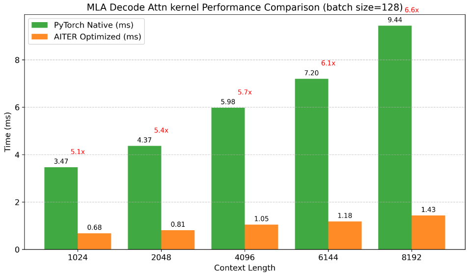
Rigorous benchmarking shows the real ability of the kernel:
Benchmark Highlights:
Evaluated multiple context lengths (512-4096 tokens)
Tested with fixed batch sizes (128)
Compared different MLA algorithm implementations
Result:
A consistent speedup over native PyTorch implementations.
Imagine what these gains could mean for your application:
Reduced latency for real-time applications
Increased throughput for batch processing
Lower compute costs across the board
Ready to take the next step? Dive deeper into the AITER capabilities with the following resources:
Explore the AITER GitHub repository.
Check out additional optimization examples.
Star the repository to stay updated on new features.