Grafana GUI analysis#
Find setup instructions in Setting up Grafana server for ROCm Compute Profiler.
The ROCm Compute Profiler Grafana analysis dashboard GUI supports the following features to facilitate MI accelerator performance profiling and analysis:
System and hardware component (hardware block)
Speed-of-Light (SOL)
Multiple normalization options
Baseline comparisons
Regex-based dispatch ID filtering
Roofline analysis
Detailed performance counters and metrics per hardware component, such as:
Command Processor - Fetch (CPF) / Command Processor - Controller (CPC)
Workgroup Manager (SPI)
Shader Sequencer (SQ)
Shader Sequencer Controller (SQC)
L1 Address Processing Unit, a.k.a. Texture Addresser (TA) / L1 Backend Data Processing Unit, a.k.a. Texture Data (TD)
L1 Cache (TCP)
L2 Cache (TCC) (both aggregated and per-channel perf info)
See the full list of ROCm Compute Profiler’s analysis panels.
Speed-of-Light#
Speed-of-Light panels are provided at both the system and per hardware component level to help diagnosis performance bottlenecks. The performance numbers of the workload under testing are compared to the theoretical maximum, such as floating point operations, bandwidth, cache hit rate, etc., to indicate the available room to further utilize the hardware capability.
Normalizations#
Multiple performance number normalizations are provided to allow performance inspection within both hardware and software context. The following normalizations are available.
per_waveper_cycleper_kernelper_second
See Normalization units to learn more about ROCm Compute Profiler normalizations.
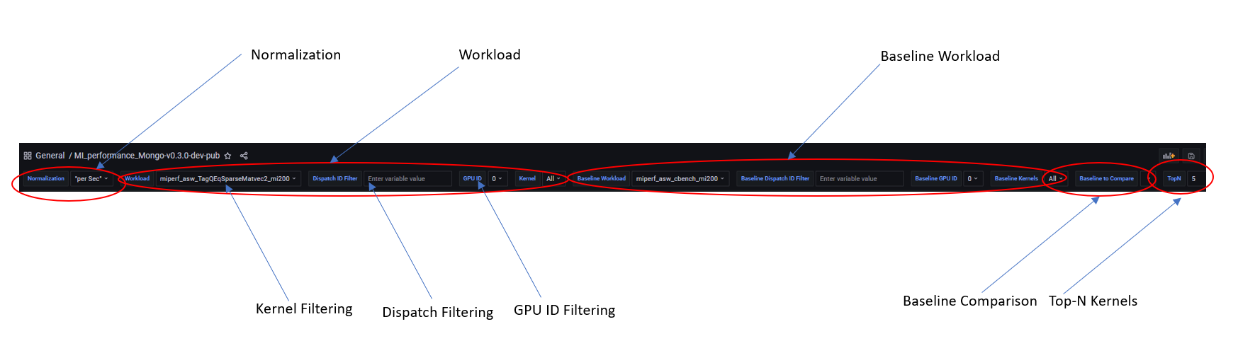
Baseline comparison#
ROCm Compute Profiler enables baseline comparison to allow checking A/B effect. Currently baseline comparison is limited to the same SoC. Cross comparison between SoCs is in development.
For both the Current Workload and the Baseline Workload, you can independently setup the following filters to allow fine grained comparisons:
Workload Name
GPU ID filtering (multi-selection)
Kernel Name filtering (multi-selection)
Dispatch ID filtering (regex filtering)
ROCm Compute Profiler Panels (multi-selection)
Regex-based dispatch ID filtering#
ROCm Compute Profiler allows filtering via Regular Expressions (regex), a standard Linux string matching syntax, based dispatch ID filtering to flexibly choose the kernel invocations.
For example, to inspect Dispatch Range from 17 to 48, inclusive, the
corresponding regex is : (1[7-9]|[23]\d|4[0-8]).
Tip
Try Regex Numeric Range Generator for help generating typical number ranges.
Incremental profiling#
ROCm Compute Profiler supports incremental profiling to speed up performance analysis.
Refer to the Hardware component filtering section for this command.
By default, the entire application is profiled to collect performance counters for all hardware blocks, giving a complete view of where the workload stands in terms of performance optimization opportunities and bottlenecks.
You can choose to focus on only a few hardware components – for example L1 cache or LDS – to closely check the effect of software optimizations, without performing application replay for all other hardware components. This saves a lot of compute time. In addition, prior profiling results for other hardware components are not overwritten; instead, they can be merged during the import to piece together an overall profile of the system.
Color coding#
Uniform color coding applies to most visualizations – including bar graphs, tables, and diagrams – for easy inspection. As a rule of thumb, yellow means over 50%, while red means over 90% percent.
Global variables and configurations#
Grafana GUI import#
The ROCm Compute Profiler database --import option imports the raw profiling data to
Grafana’s backend MongoDB database. This step is only required for Grafana
GUI-based performance analysis.
Default username and password for MongoDB (to be used in database mode) are as follows:
Username:
tempPassword:
temp123
Each workload is imported to a separate database with the following naming convention:
rocprofiler-compute_<team>_<database>_<soc>
For example:
rocprofiler-compute_asw_vcopy_mi200
When using database mode, be sure to tailor the
connection options to the machine hosting your
server-side instance. Below is the sample
command to import the vcopy profiling data, assuming our host machine is
called dummybox.
$ rocprof-compute database --help
usage:

rocprof-compute database <interaction type> [connection options]


-------------------------------------------------------------------------------

Examples:

        rocprof-compute database --import -H pavii1 -u temp -t asw -w workloads/vcopy/mi200/

        rocprof-compute database --remove -H pavii1 -u temp -w rocprofiler-compute_asw_sample_mi200

-------------------------------------------------------------------------------


Help:
  -h, --help         show this help message and exit

General Options:
  -v, --version      show program's version number and exit
  -V, --verbose      Increase output verbosity (use multiple times for higher levels)
  -s, --specs        Print system specs.

Interaction Type:
  -i, --import                                  Import workload to ROCm Compute Profiler DB
  -r, --remove                                  Remove a workload from ROCm Compute Profiler DB

Connection Options:
  -H , --host                                   Name or IP address of the server host.
  -P , --port                                   TCP/IP Port. (DEFAULT: 27018)
  -u , --username                               Username for authentication.
  -p , --password                               The user's password. (will be requested later if it's not set)
  -t , --team                                   Specify Team prefix.
  -w , --workload                               Specify name of workload (to remove) or path to workload (to import)
  --kernel-verbose              Specify Kernel Name verbose level 1-5. Lower the level, shorter the kernel name. (DEFAULT: 5) (DISABLE: 5)
ROCm Compute Profiler import for vcopy:#
$ rocprof-compute database --import -H dummybox -u temp -t asw -w workloads/vcopy/mi200/

                                 __                                       _
 _ __ ___   ___ _ __  _ __ ___  / _|       ___ ___  _ __ ___  _ __  _   _| |_ ___
| '__/ _ \ / __| '_ \| '__/ _ \| |_ _____ / __/ _ \| '_ ` _ \| '_ \| | | | __/ _ \
| | | (_) | (__| |_) | | | (_) |  _|_____| (_| (_) | | | | | | |_) | |_| | ||  __/
|_|  \___/ \___| .__/|_|  \___/|_|        \___\___/|_| |_| |_| .__/ \__,_|\__\___|
               |_|                                           |_|


Pulling data from  /home/auser/repos/rocprofiler-compute/sample/workloads/vcopy/MI200
The directory exists
Found sysinfo file
KernelName shortening enabled
Kernel name verbose level: 2
Password:
Password received
-- Conversion & Upload in Progress --
  0%|                                                                                                                                                                                                             | 0/11 [00:00<?, ?it/s]/home/auser/repos/rocprofiler-compute/sample/workloads/vcopy/MI200/SQ_IFETCH_LEVEL.csv
  9%|█████████████████▉                                                                                                                                                                                   | 1/11 [00:00<00:01,  8.53it/s]/home/auser/repos/rocprofiler-compute/sample/workloads/vcopy/MI200/pmc_perf.csv
 18%|███████████████████████████████████▊                                                                                                                                                                 | 2/11 [00:00<00:01,  6.99it/s]/home/auser/repos/rocprofiler-compute/sample/workloads/vcopy/MI200/SQ_INST_LEVEL_SMEM.csv
 27%|█████████████████████████████████████████████████████▋                                                                                                                                               | 3/11 [00:00<00:01,  7.90it/s]/home/auser/repos/rocprofiler-compute/sample/workloads/vcopy/MI200/SQ_LEVEL_WAVES.csv
 36%|███████████████████████████████████████████████████████████████████████▋                                                                                                                             | 4/11 [00:00<00:00,  8.56it/s]/home/auser/repos/rocprofiler-compute/sample/workloads/vcopy/MI200/SQ_INST_LEVEL_LDS.csv
 45%|█████████████████████████████████████████████████████████████████████████████████████████▌                                                                                                           | 5/11 [00:00<00:00,  9.00it/s]/home/auser/repos/rocprofiler-compute/sample/workloads/vcopy/MI200/SQ_INST_LEVEL_VMEM.csv
 55%|███████████████████████████████████████████████████████████████████████████████████████████████████████████▍                                                                                         | 6/11 [00:00<00:00,  9.24it/s]/home/auser/repos/rocprofiler-compute/sample/workloads/vcopy/MI200/sysinfo.csv
 64%|█████████████████████████████████████████████████████████████████████████████████████████████████████████████████████████████▎                                                                       | 7/11 [00:00<00:00,  9.37it/s]/home/auser/repos/rocprofiler-compute/sample/workloads/vcopy/MI200/roofline.csv
 82%|█████████████████████████████████████████████████████████████████████████████████████████████████████████████████████████████████████████████████████████████████▏                                   | 9/11 [00:00<00:00, 12.60it/s]/home/auser/repos/rocprofiler-compute/sample/workloads/vcopy/MI200/timestamps.csv
100%|████████████████████████████████████████████████████████████████████████████████████████████████████████████████████████████████████████████████████████████████████████████████████████████████████| 11/11 [00:00<00:00, 11.05it/s]
9 collections added.
Workload name uploaded
-- Complete! --
ROCm Compute Profiler panels#
There are currently 18 main panel categories available for analyzing the compute workload performance. Each category contains several panels for close inspection of the system performance.
-
Kernel time histogram
Top ten bottleneck kernels
-
Speed-of-Light
System Info table
-
FP32/FP64
FP16/INT8
-
Command Processor - Fetch (CPF)
Command Processor - Controller (CPC)
Workgroup Manager or Shader Processor Input (SPI)
SPI Stats
SPI Resource Allocations
-
Wavefront Launch Stats
Wavefront runtime stats
per-SE Wavefront Scheduling performance
-
Wavefront lifetime breakdown
per-SE wavefront life (average)
per-SE wavefront life (histogram)
-
per-SE wavefront occupancy
per-CU wavefront occupancy
Compute Unit - Instruction Mix
per-wave Instruction mix
per-wave VALU Arithmetic instruction mix
per-wave MFMA Arithmetic instruction mix
Compute Unit - Compute Pipeline
Speed-of-Light: Compute Pipeline
Arithmetic OPs count
Compute pipeline stats
Memory latencies
-
Speed-of-Light: LDS
LDS stats
-
Speed-of-Light: Instruction Cache
Instruction Cache Accesses
Constant Cache
Speed-of-Light: Constant Cache
Constant Cache Accesses
Constant Cache - L2 Interface stats
Texture Addresser and Texture Data
Texture Addresser (TA)
Texture Data (TD)
L1 Cache
Speed-of-Light: L1 Cache
L1 Cache Accesses
L1 Cache Stalls
L1 - L2 Transactions
L1 - UTCL1 Interface stats
-
Speed-of-Light: L2 Cache
L2 Cache Accesses
L2 - EA Transactions
L2 - EA Stalls
L2 Cache Per Channel Performance
Per-channel L2 Hit rate
Per-channel L1-L2 Read requests
Per-channel L1-L2 Write Requests
Per-channel L1-L2 Atomic Requests
Per-channel L2-EA Read requests
Per-channel L2-EA Write requests
Per-channel L2-EA Atomic requests
Per-channel L2-EA Read latency
Per-channel L2-EA Write latency
Per-channel L2-EA Atomic latency
Per-channel L2-EA Read stall (I/O, GMI, HBM)
Per-channel L2-EA Write stall (I/O, GMI, HBM, Starve)
Most panels are designed around a specific hardware component block to thoroughly understand its behavior. Additional panels, including custom panels, could also be added to aid the performance analysis.
System Info#
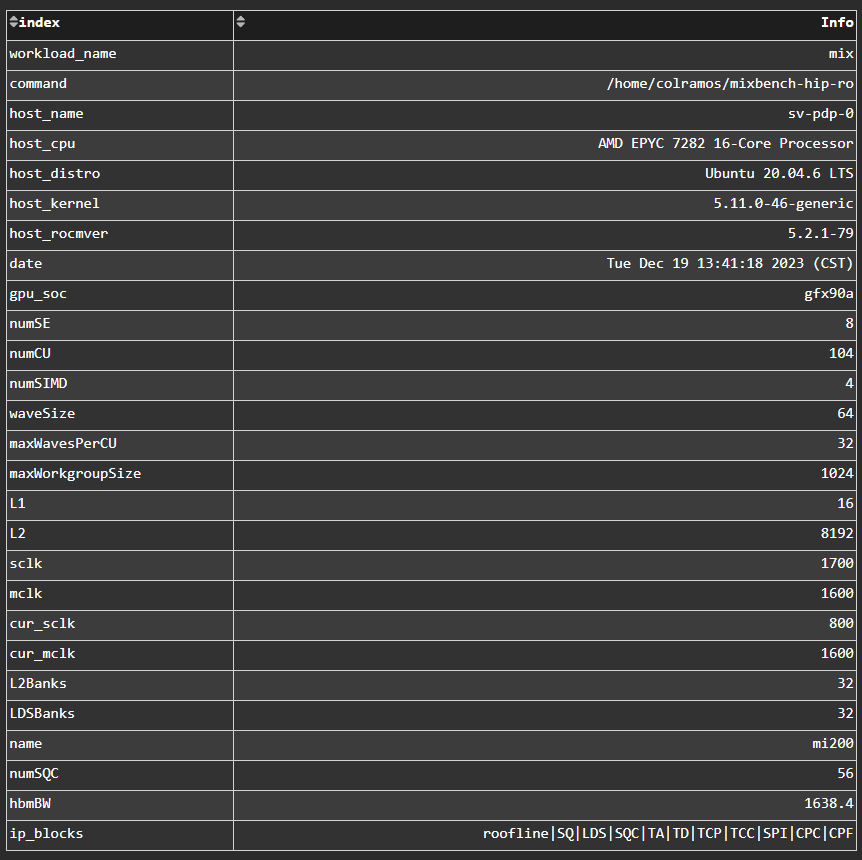
Fig. 7 System details logged from the host machine.#
Kernel Statistics#
Kernel Time Histogram#
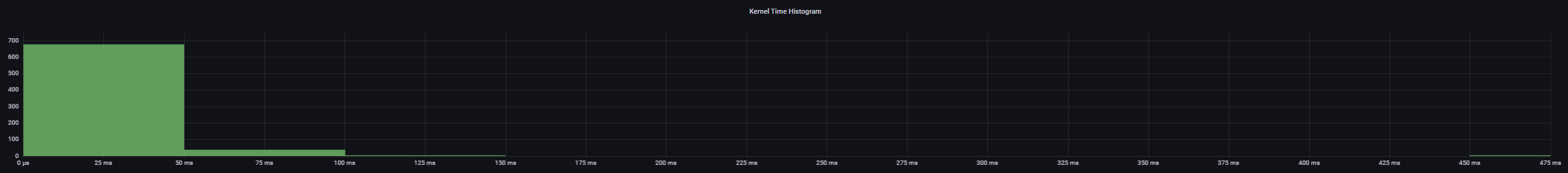
Fig. 8 Mapping application kernel launches to execution duration.#
Top Bottleneck Kernels#
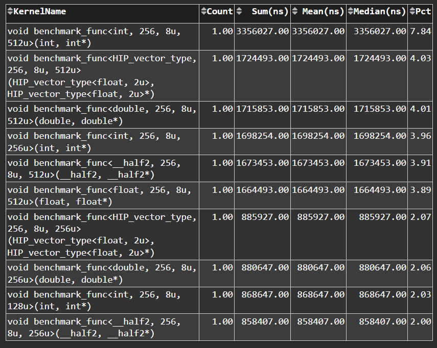
Fig. 9 Top N kernels and relevant statistics. Sorted by total duration.#
Top Bottleneck Dispatches#
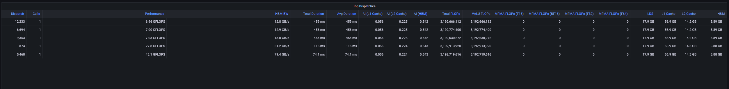
Fig. 10 Top N kernel dispatches and relevant statistics. Sorted by total duration.#
Current and Baseline Dispatch IDs (Filtered)#
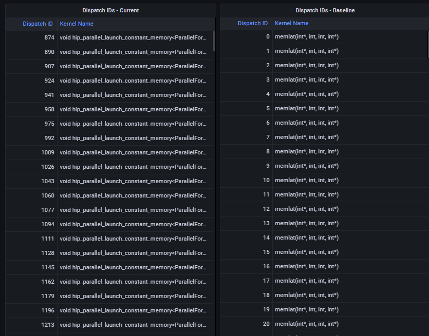
Fig. 11 List of all kernel dispatches.#
System Speed-of-Light#
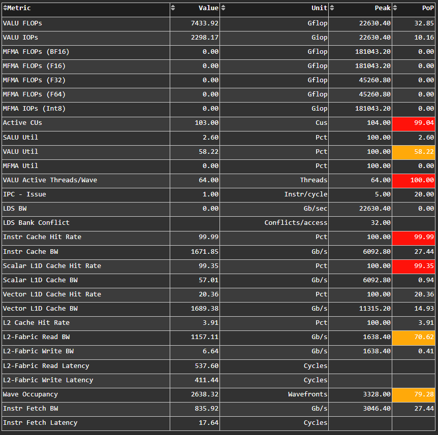
Fig. 12 Key metrics from various sections of ROCm Compute Profiler’s profiling report.#
Tip
See System Speed-of-Light to learn about reported metrics.
Memory Chart Analysis#
Note
The Memory Chart Analysis support multiple normalizations. Due to limited
space, all transactions, when normalized to per_sec, default to unit of
billion transactions per second.
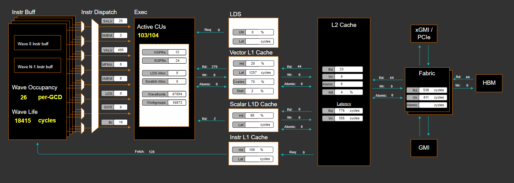
Fig. 13 A graphical representation of performance data for memory blocks on the GPU.#
Empirical Roofline Analysis#
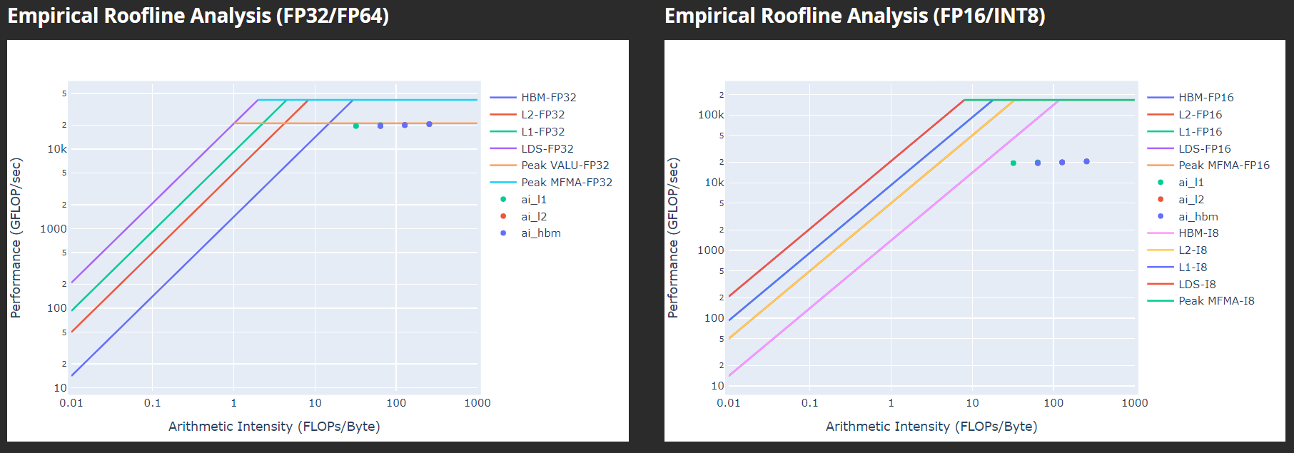
Fig. 14 Visualize achieved performance relative to a benchmarked peak performance.#
Command Processor#
Tip
See Command processor (CP) to learn about reported metrics.
Command Processor Fetcher#
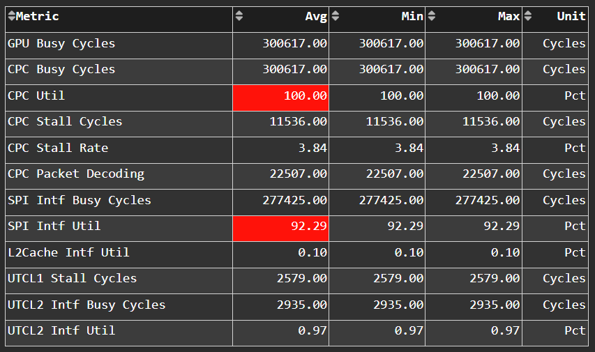
Fig. 15 Fetches commands out of memory to hand them over to the Command Processor Fetcher (CPC) for processing#
Command Processor Compute#
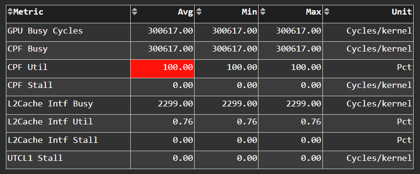
Fig. 16 The micro-controller running the command processing firmware that decodes the fetched commands, and (for kernels) passes them to the Workgroup Managers (SPIs) for scheduling.#
Shader Processor Input (SPI)#
Tip
See Workgroup manager (SPI) to learn about reported metrics.
SPI Stats#
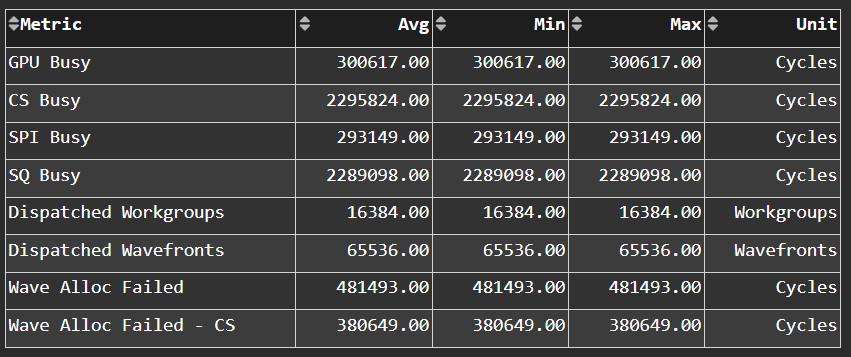
SPI Resource Allocation#
Wavefront#
Wavefront Launch Stats#
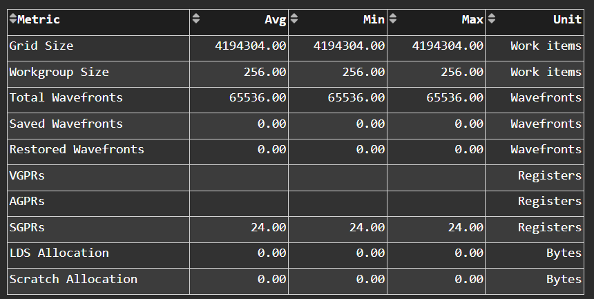
Fig. 17 General information about the kernel launch.#
Tip
See Wavefront launch stats to learn about reported metrics.
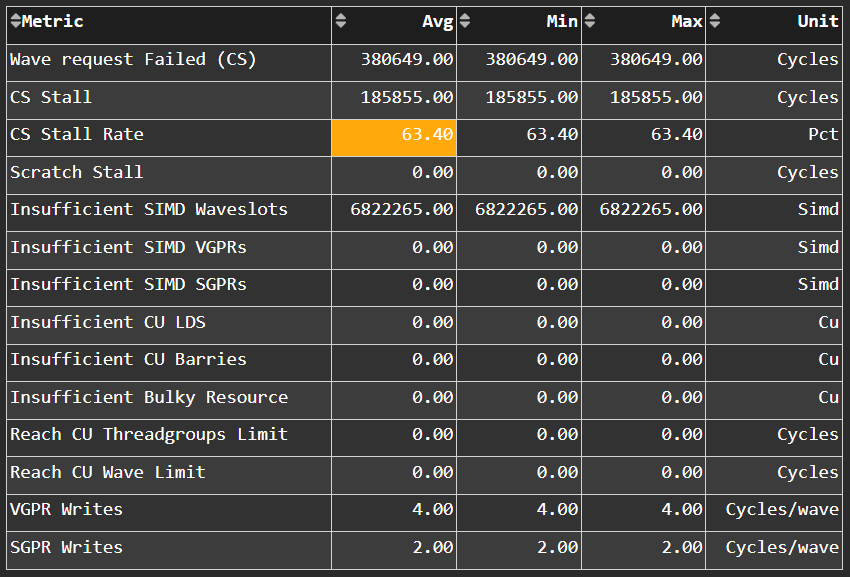
Wavefront Runtime Stats#
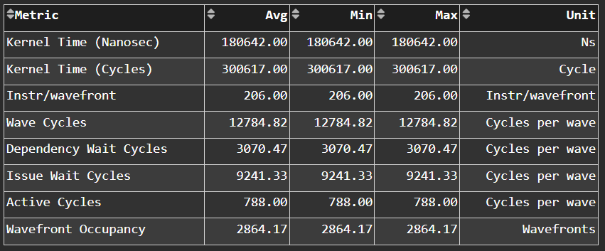
Fig. 18 High-level overview of the execution of wavefronts in a kernel.#
Tip
See Wavefront runtime stats to learn about reported metrics.
Compute Unit - Instruction Mix#
Instruction Mix#
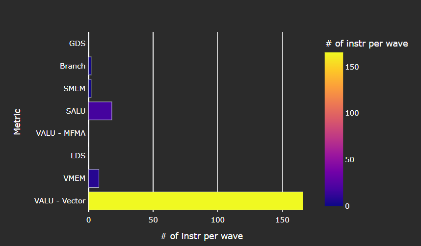
Fig. 19 Breakdown of the various types of instructions executed by the user’s kernel, and which pipelines on the Compute Unit (CU) they were executed on.#
Tip
See Instruction mix to learn about reported metrics.
VALU Arithmetic Instruction Mix#
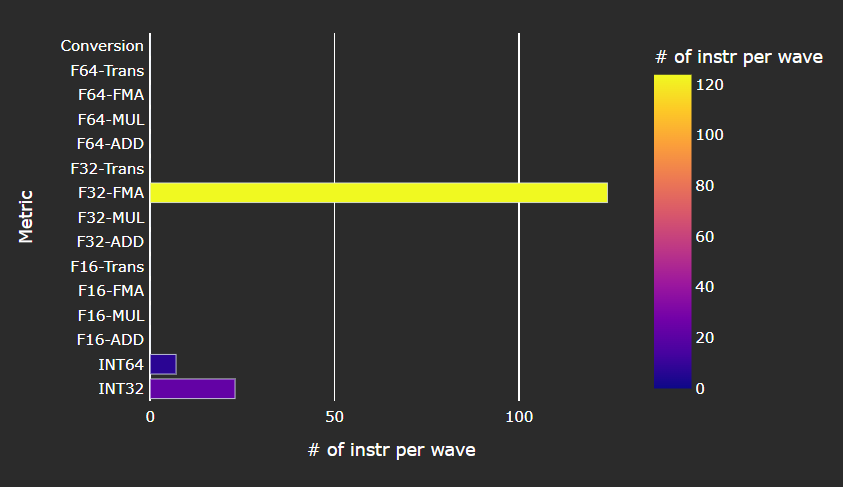
Fig. 20 The various types of vector instructions that were issued to the vector arithmetic logic unit (VALU).#
Tip
See VALU arithmetic instruction mix to learn about reported metrics.
MFMA Arithmetic Instruction Mix#
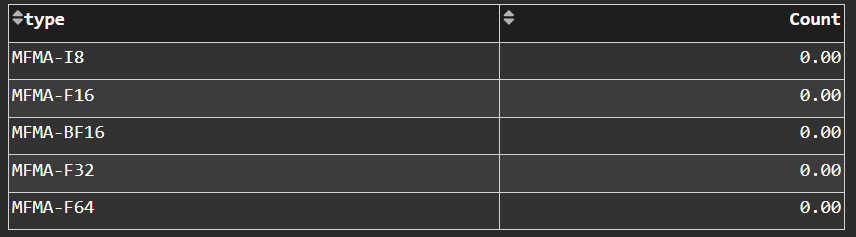
Fig. 21 The types of Matrix Fused Multiply-Add (MFMA) instructions that were issued.#
Tip
See MFMA instruction mix to learn about reported metrics.
VMEM Arithmetic Instruction Mix#
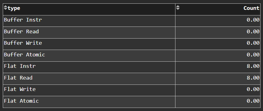
Fig. 22 The types of vector memory (VMEM) instructions that were issued.#
Tip
See VMEM instruction mix to learn about reported metrics.
Compute Unit - Compute Pipeline#
Speed-of-Light#
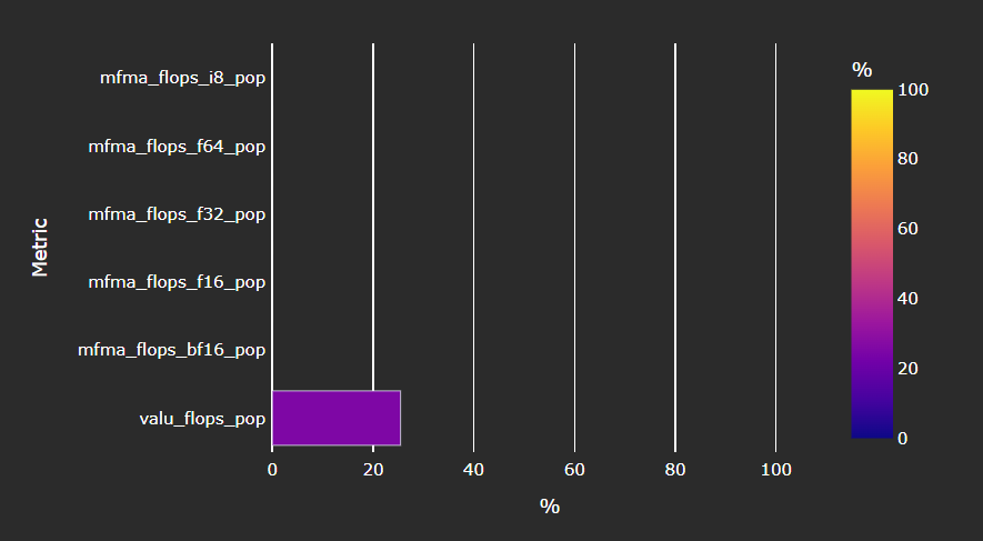
Fig. 23 The number of floating-point and integer operations executed on the vector arithmetic logic unit (VALU) and Matrix Fused Multiply-Add (MFMA) units in various precisions.#
Tip
See Compute Speed-of-Light to learn about reported metrics.
Pipeline Stats#
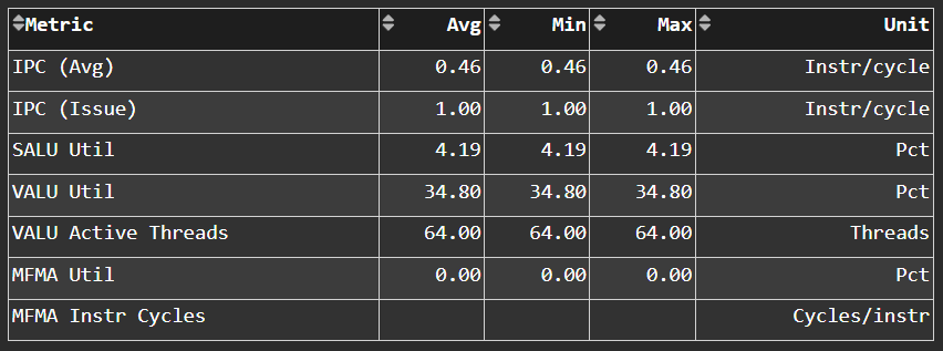
Fig. 24 More detailed metrics to analyze the several independent pipelines found in the Compute Unit (CU).#
Tip
See Pipeline statistics to learn about reported metrics.
Arithmetic Operations#
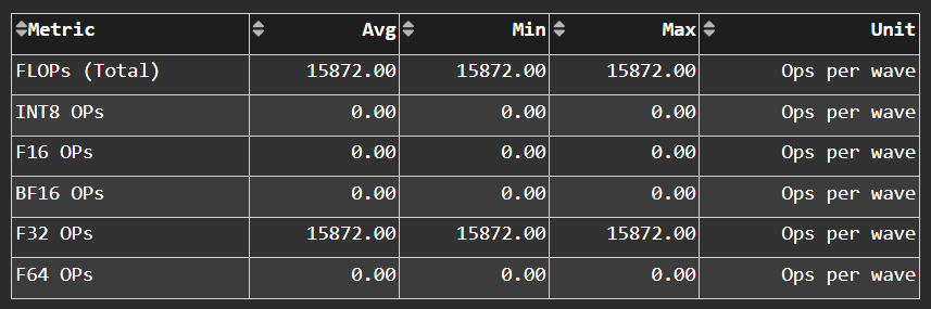
Fig. 25 The total number of floating-point and integer operations executed in various precisions.#
Tip
See Arithmetic operations to learn about reported metrics.
Local Data Share (LDS)#
Speed-of-Light#
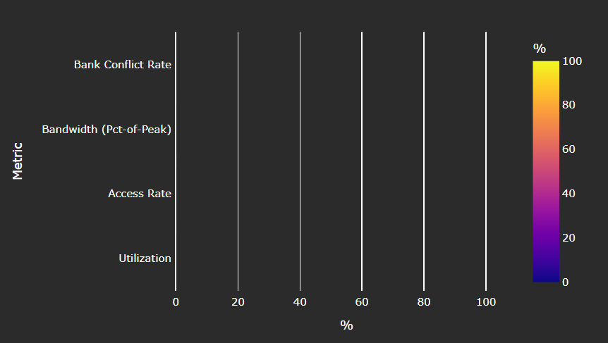
Fig. 26 Key metrics for the Local Data Share (LDS) as a comparison with the peak achievable values of those metrics.#
Tip
See LDS Speed-of-Light to learn about reported metrics.
LDS Stats#
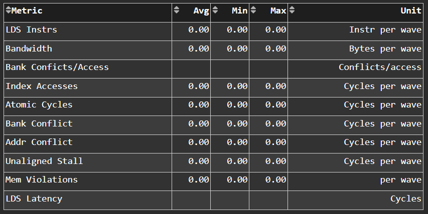
Fig. 27 More detailed view of the Local Data Share (LDS) performance.#
Tip
See Statistics to learn about reported metrics.
Instruction Cache#
Speed-of-Light#
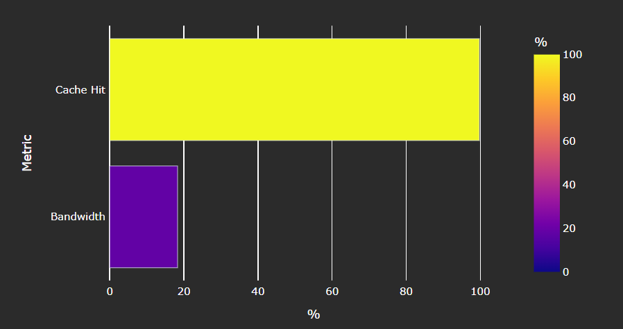
Fig. 28 Key metrics of the L1 Instruction (L1I) cache as a comparison with the peak achievable values of those metrics.#
Tip
See L1I Speed-of-Light to learn about reported metrics.
Instruction Cache Stats#
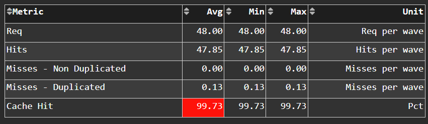
Fig. 29 More detail on the hit/miss statistics of the L1 Instruction (L1I) cache.#
Tip
See L1I cache accesses to learn about reported metrics.
Scalar L1D Cache#
Tip
See Scalar L1 data cache (sL1D) to learn about reported metrics.
Speed-of-Light#
Fig. 30 Key metrics of the Scalar L1 Data (sL1D) cache as a comparison with the peak achievable values of those metrics.#
Tip
See Scalar L1D Speed-of-Light to learn about reported metrics.
Scalar L1D Cache Accesses#
Fig. 31 More detail on the types of accesses made to the Scalar L1 Data (sL1D) cache, and the hit/miss statistics.#
Tip
See Scalar L1D cache accesses to learn about reported metrics.
Scalar L1D Cache - L2 Interface#
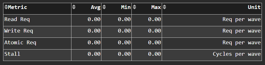
Fig. 32 More detail on the data requested across the Scalar L1 Data (sL1D) cache <-> L2 interface.#
Tip
See sL1D ↔ L2 Interface to learn about reported metrics.
Texture Address and Texture Data#
Texture Addresser#
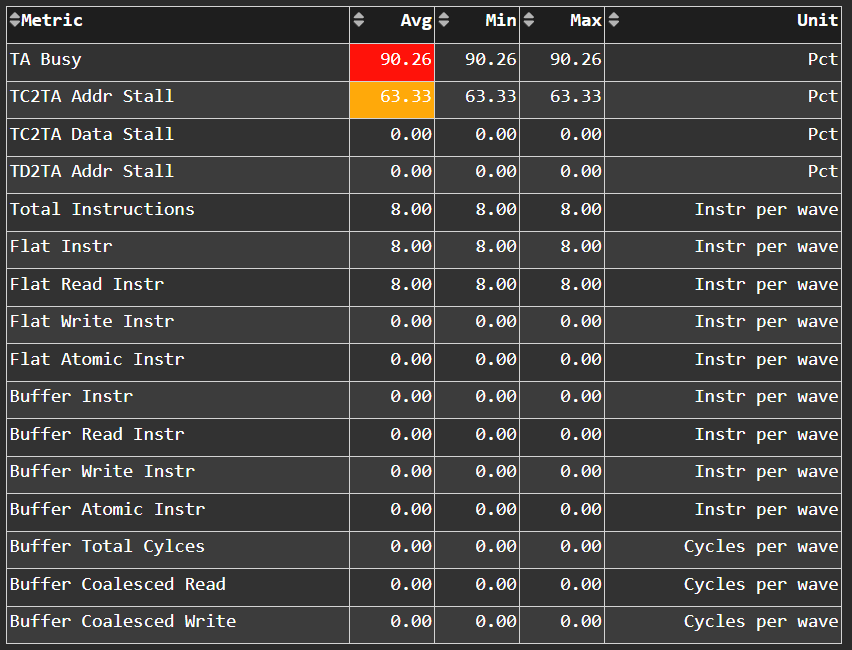
Fig. 33 Metric specific to texture addresser (TA) which receives commands (e.g., instructions) and write/atomic data from the Compute Unit (CU), and coalesces them into fewer requests for the cache to process.#
Tip
See Address processing unit or Texture Addresser (TA) to learn about reported metrics.
Texture Data#
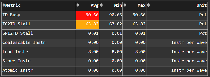
Fig. 34 Metrics specific to texture data (TD) which routes data back to the requesting Compute Unit (CU).#
Tip
See Vector L1 data-return path or Texture Data (TD) to learn about reported metrics.
Vector L1 Data Cache#
Speed-of-Light#
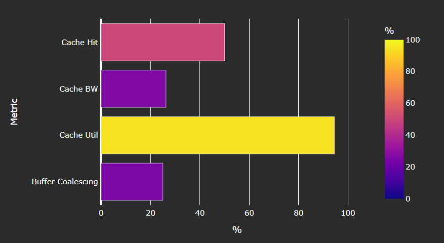
Fig. 35 Key metrics of the vector L1 data (vL1D) cache as a comparison with the peak achievable values of those metrics.#
Tip
See vL1D Speed-of-Light to learn about reported metrics.
L1D Cache Stalls#
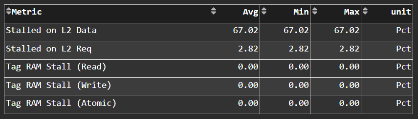
Fig. 36 More detail on where vector L1 data (vL1D) cache is stalled in the pipeline, which may indicate performance limiters of the cache.#
Tip
See vL1D cache stall metrics to learn about reported metrics.
L1D Cache Accesses#
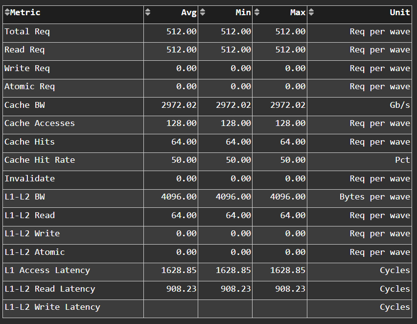
Fig. 37 The type of requests incoming from the cache front-end, the number of requests that were serviced by the vector L1 data (vL1D) cache, and the number & type of outgoing requests to the L2 cache.#
Tip
See vL1D cache access metrics to learn about reported metrics.
L1D - L2 Transactions#
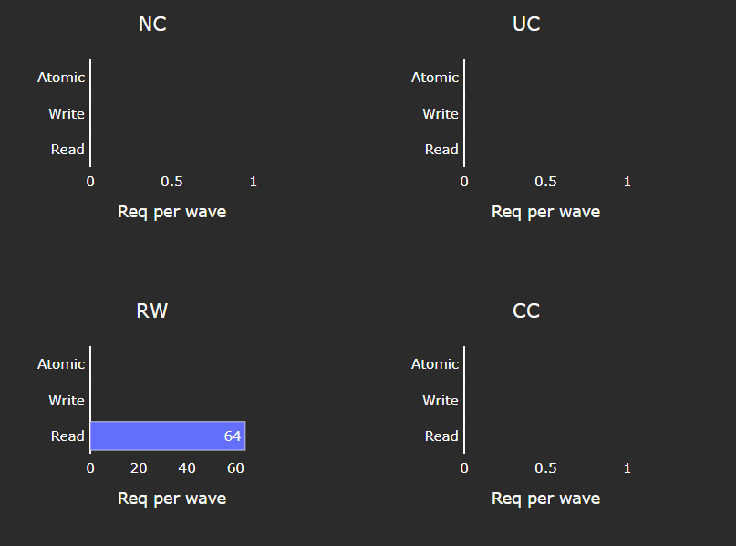
Fig. 38 A more granular look at the types of requests made to the L2 cache.#
Tip
See vL1D - L2 Transaction Detail to learn more.
L1D Addr Translation#
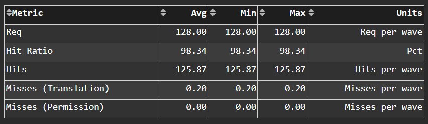
Fig. 39 After a vector memory instruction has been processed/coalesced by the address processing unit of the vector L1 data (vL1D) cache, it must be translated from a virtual to physical address. These metrics provide more details on the L1 Translation Lookaside Buffer (TLB) which handles this process.#
Tip
See L1 Unified Translation Cache (UTCL1) to learn about reported metrics.
L2 Cache#
Tip
See L2 cache (TCC) to learn about reported metrics.
Speed-of-Light#
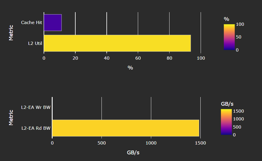
Fig. 40 Key metrics about the performance of the L2 cache, aggregated over all the L2 channels, as a comparison with the peak achievable values of those metrics.#
Tip
See L2 Speed-of-Light to learn about reported metrics.
L2 Cache Accesses#
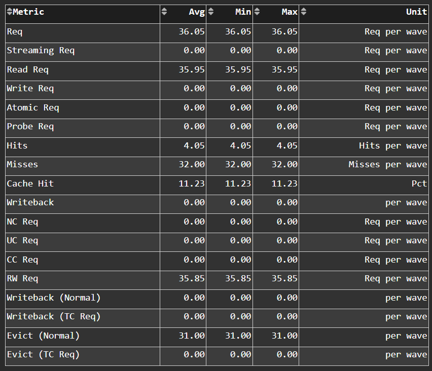
Fig. 41 Incoming requests to the L2 cache from the vector L1 data (vL1D) cache and other clients (e.g., the sL1D and L1I caches).#
Tip
See L2 cache accesses to learn about reported metrics.
L2 - Fabric Transactions#
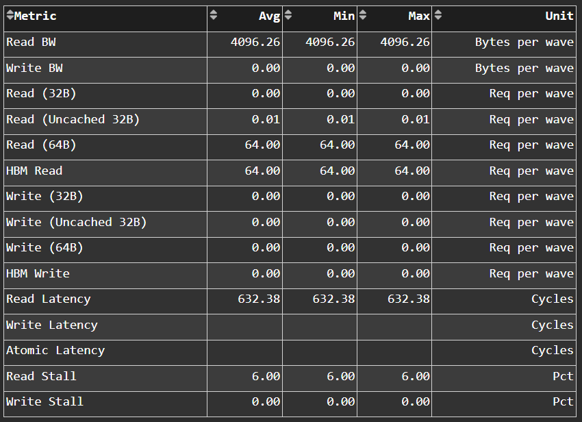
Fig. 42 More detail on the flow of requests through Infinity Fabric™.#
Tip
See L2-Fabric transactions to learn about reported metrics.
L2 - Fabric Interface Stalls#
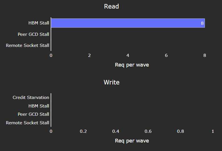
Fig. 43 A breakdown of what types of requests in a kernel caused a stall (e.g., read vs write), and to which locations (e.g., to the accelerator’s local memory, or to remote accelerators/CPUs).#
Tip
See L2-Fabric interface stalls to learn about reported metrics.
L2 Cache Per Channel#
Tip
See L2 Speed-of-Light for more information.
Aggregate Stats#
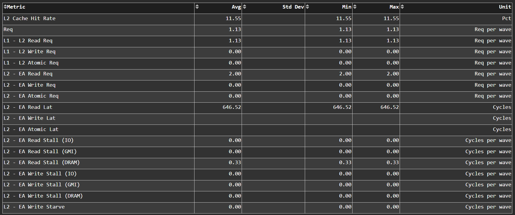
Fig. 44 L2 Cache per channel performance at a glance. Metrics are aggregated over all available channels.#