Optimizing with Composable Kernel

Optimizing with Composable Kernel#

Applies to Linux

2024-06-05

26 min read time

The AMD ROCm™ Composable Kernel (CK) library provides a programming model for writing performance-critical kernels for machine learning workloads. It generates a general-purpose kernel during the compilation phase through a C++ template, enabling developers to achieve operation fusions on different data precisions.

This article gives a high-level overview of CK General Matrix Multiplication (GEMM) kernel based on the design example of 03_gemm_bias_relu. It also outlines the steps to construct the kernel and run it. Moreover, the article provides a detailed implementation of running SmoothQuant quantized INT8 models on AMD Instinct MI300X accelerators using CK.

High-level overview: a CK GEMM instance#

GEMM is a fundamental block in linear algebra, machine learning, and deep neural networks. It is defined as the operation: \(E = α \times (A \times B) + β \times (D)\), with A and B as matrix inputs, α and β as scalar inputs, and D as a pre-existing matrix. Take the commonly used linear transformation in a fully connected layer as an example. These terms correspond to input activation (A), weight (B), bias (D), and output (E), respectively. The example employs a DeviceGemmMultipleD_Xdl_CShuffle struct from CK library as the fundamental instance to explore the compute capability of AMD Instinct accelerators for the computation of GEMM. The implementation of the instance contains two phases:

Template parameter definition
Instantiating and running the templated kernel

Template parameter definition#

The template parameters of the instance are grouped into four parameter types:

Parameters for determining matrix data precision
Parameters for determining matrix data layout
Parameters for determining extra operations on matrix elements
Performance-oriented tunable parameters

../../_images/ck-template_parameters.jpg — Fig. 2 The template parameters of the selected GEMM kernel are classified into four groups. These template parameter groups should be defined properly before running the instance.#

Matrix data precision#

A, B, D, and E are defined as half-precision floating-point datatypes. The multiply-add results of matrix A and B are added with a pre-existing matrix D (half-precision), and the final GEMM results are also half-precision floating-points.

using ADataType        = F16;
using BDataType        = F16;
using AccDataType      = F32;
using CShuffleDataType = F16;
using DDataType        = F16;
using EDataType        = F16;

ADataType and BDataType denote the data precision of the A and B input matrices. AccDataType determines the data precision used for representing the multiply-add results of A and B elements. These results are stored in a CShuffle module in local data share (LDS), a low-latency and high-bandwidth explicitly-addressed memory used for synchronization within a workgroup LDS for later use.

CShuffleDataType denotes the data precision of CShuffle in LDS.

DDataType denotes the data precision of the pre-existing D matrix stored in GPU global memory, while EDatatype denotes the data precision of the final output. The CK kernel supports a fusion strategy so that CShuffle can be added with a single pre-existing matrix in the same GPU kernel for better performance.

Matrix data layout#

using ALayout = Row;
using BLayout = Col;
using DLayout = Row;
using ELayout = Row;

Following the convention of various linear algebra libraries, CK assumes that the input matrix A is an M x K matrix, meaning the matrix has M rows and K columns. Similarly, matrix B is assumed to be K x N, meaning it has K rows and N columns. In computing, row-major order and column-major order are commonly used ways to store matrices in linear storage. After understanding the matrix storage pattern, the underlying optimized memory access manner can be applied to achieve better performance depending on the storage ordering of these matrices.

Matrix element operation#

using AElementOp   = PassThrough;
using BElementOp   = PassThrough;
using CDEElementOp = AddRelu;

CK supports the pre-processing of the matrix before calculating GEMM, that is, C = AElementOp(A) * BElementOp(B). It similarly supports the post-processing of GEMM results the same way, that is, E = CDEElementOp(C, D).

AElementOp and BElementOp determine the operation applied to matrix A and B separately before GEMM, which is achieved by binding the operation with a C++ struct function.

The above PassThrough denotes no operations are performed on the target matrix. CDEELementOp determines the operations applied to CShuffle output and matrix D. The following binding struct AddRelu shows an example of adding the CShuffle output and matrix D, and ReLU (Rectified Linear Unit) operations to the addition result. It then passes the results to matrix E.

struct AddRelu
{
    __host__ __device__ void operator()(ck::half_t& e, const ck::half_t& c, const ck::half_t& d) const
    {
        const ck::half_t x = c + d;
        e = x > 0 ? x : 0;
    }
};

Tunable parameters#

The CK instance includes a series of tunable template parameters to control the parallel granularity of the workload to achieve load balancing on different hardware platforms.

These parameters include Block Size, M/N/K Per Block, M/N per XDL, AK1, BK1, etc.

Block Size determines the number of threads in the thread block.
M/N/K Per Block determines the size of tile that each thread block is responsible for calculating.
M/N Per XDL refers to M/N size for Instinct accelerator Matrix Fused Multiply Add (MFMA) instructions operating on a per-wavefront basis.
A/B K1 is related to the data type. It can be any value ranging from 1 to K Per Block. To achieve the optimal load/store performance, 128bit per load is suggested. In addition, the A/B loading parameters must be changed accordingly to match the A/B K1 value; otherwise, it will result in compilation errors.

Conditions for achieving computational load balancing on different hardware platforms can vary.

Instantiating and running the templated kernel#

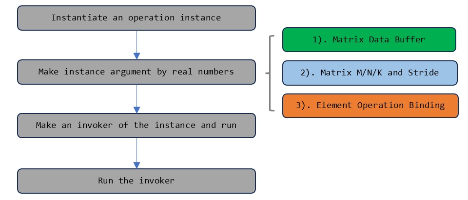
After determining the template parameters, we instantiate the kernel with actual arguments. Do one of the following:

Use GetDeviceBuffer from CK’s custom struct DeviceMem to pass the element values of the matrices that need to be calculated.
Allocate device buffer via hipMalloc. Ensure the device buffer size can fit the matrix size.
Pass matrix elements through the data_ptr method in the Tensor object if the matrix to be calculated is of Tensor type.

The row and column, and stride information of input matrices are also passed to the instance. For batched GEMM, you must pass in additional batch count and batch stride values. The extra operations for pre and post-processing are also passed with an actual argument; for example, α and β for GEMM scaling operations. Afterward, the instantiated kernel is launched by the invoker, as illustrated in Figure 3.

../../_images/ck-kernel_launch.jpg — Fig. 3 Templated kernel launching consists of kernel instantiation, making arguments by passing in actual application parameters, creating an invoker, and running the instance through the invoker.#

Developing fused INT8 kernels for SmoothQuant models#

SmoothQuant (SQ) is a quantization algorithm that enables an INT8 quantization of both weights and activations for all the matrix multiplications in LLM. The required GPU kernel functionalities used to accelerate the inference of SQ models on Instinct accelerators are shown in the following table.

Table 1 Functionalities used to implement SmoothQuant model inference.#
Functionality descriptions	Corresponding wrappers
\(E = α \times (A \times B) + β \times (D)\), where A, B, D, E are INT8 2-D tensors;	E = Linear_ABDE_I8(A, B, D, \(\alpha\), \(\beta\))
\(E = RELU (α \times (A \times B) + β \times (D))\), where A, B, D, E are INT8 2-D tensors;	E = Linear_ReLU_ABDE_I8(A, B, D, \(\alpha\), \(\beta\))
\(E = α \times (A \times B) + β \times (D)\), where A, B are INT8 2-D tensors, D and E are FP32 2-D tensors;	E = Linear_AB_I8_DE_F32(A, B, D, \(\alpha\), \(\beta\))
\(E = α \times (A \times B)\), where A, B, E are INT8 3-D tensors;	E = BMM_ABE_I8(A, B, \(\alpha\))
\(E = α \times (A \times B)\), where A, B are INT8 3-D tensors, E is FP32 3-D tensor;	E = BMM_AB_I8_E_F32(A, B, \(\alpha\))

Operation flow analysis#

The following section discusses the analysis of the operation flow of Linear_ReLU_ABDE_I8. The rest of the wrappers in Table 1 can be analyzed similarly.

The first operation in the process is to perform the multiplication of input matrices A and B. The resulting matrix C is then scaled with α to obtain T1. At the same time, the process performs a scaling operation on D elements to obtain T2. Afterward, the process performs matrix addition between T1 and T2, element activation calculation using ReLU, and element rounding sequentially. The operations to generate E1, E2, and E are encapsulated and completed by a user-defined template function in CK (given in the next sub-section). This template function is integrated into the fundamental instance directly during the compilation phase so that all these steps can be fused in a single GPU kernel.

../../_images/ck-operation_flow.jpg — Fig. 4 Operation flow.#

The CK library contains many fundamental instances that implement different functions. Familiarize yourself with the names of various CK instances and determine whether they meet the target functional requirements.

Second, consider whether the format of input data meets your actual calculation needs. For SQ models, the 8-bit integer data format (INT8) is applied for matrix calculations.

Third, consider the platform for implementing CK instances. The instances suffixed with xdl only run on AMD Instinct accelerators after being compiled and cannot run on Radeon-series GPUs. This is due to the underlying device-specific instruction sets for implementing these basic instances.

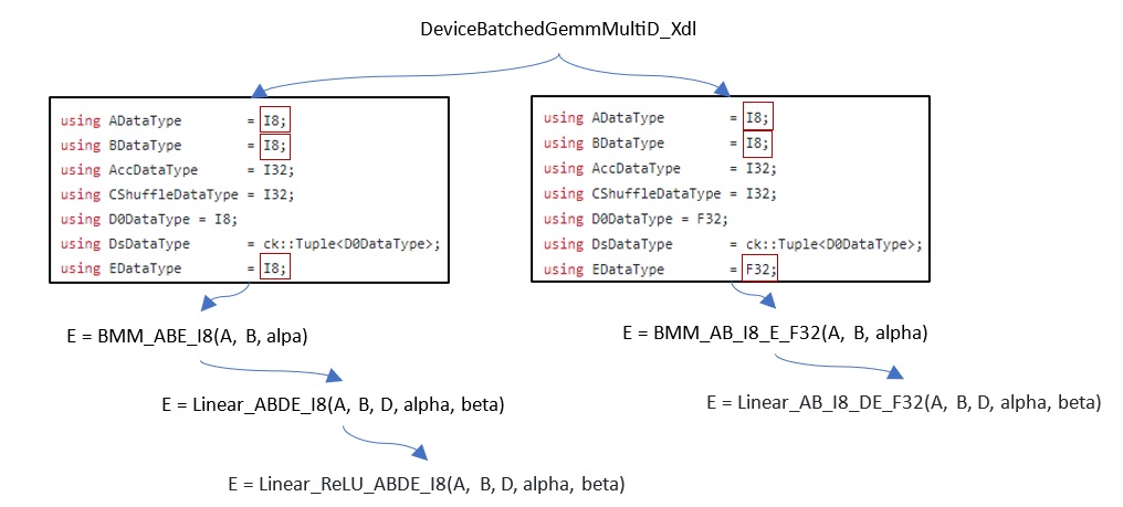
Here, we use DeviceBatchedGemmMultiD_Xdl as the fundamental instance to implement the functionalities in the previous table.

../../_images/ck-root_instance.jpg — Fig. 5 Use the ‘DeviceBatchedGemmMultiD_Xdl’ instance as a root.#

The DeviceBatchedGemmMultiD_Xdl instance realizes the batched GEMM BMM_ABE_I8 and BMM_AB_I8_E_F32 kernels directly by using the proper input and output data precision types.

Based on the two batched GEMM kernels, GEMM kernel Linear_ABDE_I8 and Linear_AB_I8_DE_F32 can be implemented by expanding their input 2-D tensors to 3-D tensors. Then, the 3-D output tensors produced by the root instance are squeezed back to 2-D output tensors before returning back.

For example, unsqueeze A (M, K) to A (1, M, K) before assigning it into the root instance and squeeze E (1, M, N) to (M, N) after the calculations of the root instance return back. Linear_ReLU_ABDE_I8 is implemented by adding a ReLU operation on the result output of Linear_ABDE_I8.

Developing the complete function#

The inference of SQ quantized models relies on using PyTorch and Transformer libraries, and a tensor type is used to represent matrices and vectors in torch, the C++ data types in CK need to be replaced with the torch::tensor type. The data types of the input and output matrices should be a tensor type.

In GEMM, the A and B inputs are two-dimensional matrices, and the required input matrices of the selected fundamental CK instance are three-dimensional matrices. Therefore, we must convert the input 2-D tensors to 3-D tensors, by using tensor’s unsqueeze() method before passing these matrices to the instance. For batched GEMM in the preceding table, ignore this step.

// Function input and output 
torch::Tensor linear_relu_abde_i8(
    torch::Tensor A_,
    torch::Tensor B_,
    torch::Tensor D_,
    float alpha,
    float beta)
{
  // Convert torch::Tensor A_ (M, K) to torch::Tensor A (1, M, K) 
  auto A = A_.unsqueeze(0);

  // Convert torch::Tensor B_ (K, N) to torch::Tensor A (1, K, N) 
  auto B = B_.unsqueeze(0);
...

As shown in the following code block, we obtain M, N, and K values using input tensor size values. This stride size information is used to reshape the input vector D and allocate the storage space of tensor E. Stride reflects the exact size of continuous elements in memory, which are passed as important parameters to the fundamental instance for GPU kernel use.

  // Return the batch count from the size of dimension 0
  int batch_count = A.size(0);

  // Return the M, N, K from the size of dimension 1 & 2
  int M = A.size(1);
  int N = B.size(1);
  int K = A.size(2);

  // Initialize the stride size for A, B, D and E
  int stride_A = K;
  int stride_B = K;
  int stride_D0 = N;
  int stride_E = N;

  // Initialize the stride size for batched A, B, D and E
  long long int batch_stride_A = M * K;
  long long int batch_stride_B = K * N;
  long long int batch_stride_D0 = M * N;
  long long int batch_stride_E = M * N;

  // Convert the tensor of 2-D to 3-D
  auto D = D_.view({1,-1}).repeat({M, 1});

  // Allocate memory for E
  auto E = torch::empty({batch_count, M, N}, 
       torch::dtype(torch::kInt8).device(A.device()));

In the following code block, ADataType, BDataType and D0DataType are used to denote the data precision of the input tensors A, B and D, respectively. EDataType is used to denote the data precision of output tensor E. These parameters are specified to I8 data format (8-bit integer data format) to meet the kernel’s design requirements.

AccDataType determines the data precision used to represent the multiply-add results of A and B elements. Generally, a larger range data type is applied to store the multiply-add results of A and B to avoid result overflow; I32 is applied in this case. The CShuffleDataType I32 data type indicates that the multiply-add results continue to be stored in LDS as an I32 data format. All of this is implemented through the following code block.

  // Data precision 
  using ADataType        = I8;
  using BDataType        = I8;
  using AccDataType      = I32;
  using CShuffleDataType = I32;
  using D0DataType       = I8;
  using DsDataType       = ck::Tuple<D0DataType>;
  using EDataType        = I8;

Following the convention of various linear algebra libraries, row-major and column-major orders are used to denote the ways of storing matrices in linear storage. The advantage of specifying matrix B as column major is that all the relevant matrix elements are stored continuously in GPU global memory when a row in A is multiplied by a column in B, which can help GPU achieve data consistency access to improve access performance.

  // Specify tensor order
  using ALayout  = RowMajor;
  using BLayout  = ColumnMajor;
  using D0Layout = RowMajor;
  using DsLayout = ck::Tuple<D0Layout>;
  using ELayout  = RowMajor;

In CK, PassThrough is a struct denoting if an operation is applied to the tensor it binds to. To fuse the operations between E1, E2, and E introduced in section Operation flow analysis, we define a custom C++ struct, ScaleScaleAddRelu, and bind it to CDEELementOp. It determines the operations that will be applied to CShuffle (A×B results), tensor D, α, and β.

  // No operations bound to the elements of A and B 
  using AElementOp   = PassThrough;
  using BElementOp   = PassThrough;

  // Operations bound to the elements of C, D and E
  using CDEElementOp = ScaleScaleAddRelu;

In the binding struct, operator() performs an addition operation between CShuffle and matrix D, a ReLU operation on the addition results, and a rounding operation on the output elements. It then returns the results to E.

struct ScaleScaleAddRelu {

  template <>
  __host__ __device__ constexpr void
  operator()<I8, I32, I8>(I8& e, const I32& c, const I8& d) const
  {
      // Scale AxB result with alpha
      const F32 c_scale = ck::type_convert<F32>(c) * alpha;

      // Scale D with beta
      const F32 d_scale = ck::type_convert<F32>(d) * beta;

      // Perform addition operation
      F32 temp = c_scale + d_scale;
      
      // Perform RELU operation
      temp = temp > 0 ? temp : 0;

      // Perform rounding operation 
      temp = temp > 127 ? 127 : temp;
      
      // Return to E
      e = ck::type_convert<I8>(temp);
  }
    
  F32 alpha;
  F32 beta;
};

The original input tensors need to be padded to meet GPU tile-based parallelism.

static constexpr auto GemmDefault = ck::tensor_operation::device::GemmSpecialization::MNKPadding;

The template parameters of the target fundamental instance are initialized with the above parameters and includes default tunable parameters. For specific tuning methods, see Tunable parameters.

using DeviceOpInstance = ck::tensor_operation::device::DeviceBatchedGemmMultiD_Xdl< 
    // Tensor layout
    ALayout, BLayout, DsLayout, ELayout, 
    // Tensor data type
    ADataType, BDataType, AccDataType, CShuffleDataType, DsDataType, EDataType,  
    // Tensor operation
    AElementOp,  BElementOp, CDEElementOp,  
    // Padding strategy  
    GemmDefault,
    // Tunable parameters        
    tunable parameters>;

Return the address of the first element of tensors:

 auto A_ref = A.data_ptr<ADataType>();
 auto B_ref = B.data_ptr<BDataType>();
 auto D0_ref = D.data_ptr<D0DataType>();
 auto E_ref = E.data_ptr<EDataType>();

The fundamental instance is then initialized and run with actual arguments:

 auto device_op    = DeviceOpInstance{};
 auto invoker = device_op.MakeInvoker();
 auto argument = device_op.MakeArgument(
    A_ref, B_ref, {D0_ref}, E_ref,
    M, N, K,
    batch_count,
    stride_A, stride_B, {stride_D0}, stride_E,
    batch_stride_A, batch_stride_B, {batch_stride_D0}, batch_stride_E,
    AElementOp{}, BElementOp{}, CDEElementOp{alpha, beta});

invoker.Run(argument, StreamConfig{nullptr, 0});

The output of the fundamental instance is a calculated batched matrix E (batch, M, N). Before the return, it needs to be converted to a 2-D matrix if a normal GEMM result is required.

// Convert (1, M, N) to (M, N) 
return E.squeeze(0);

Binding to Python#

Since these functions are written in C++ and torch::Tensor, you can use pybind11 to bind the functions and import them as Python modules. For the example, the necessary binding code for exposing the functions in the table spans but a few lines.

#include <torch/extension.h>

PYBIND11_MODULE(TORCH_EXTENSION_NAME, m){
  m.def("linear_ab_i8_de_f32", &linear_ab_i8_de_f32);
  m.def("linear_relu_abde_i8", &linear_relu_abde_i8);
  m.def("linear_abde_i8", &linear_abde_i8);
  m.def("bmm_abe_i8", &bmm_abe_i8);
  m.def("bmm_ab_i8_e_f32", &bmm_ab_i8_e_f32);
}

Build the C++ extension by writing a setup.py script that uses setuptools to compile the C++ code. A reference implementation of the setup.py script is as follows.

import os
from setuptools import setup, find_packages
from torch.utils import cpp_extension
from torch.utils.cpp_extension import BuildExtension

os.environ["CC"] = "hipcc"
os.environ["CXX"] = "hipcc"

sources = [
    'torch_int/kernels/linear.cpp',
    'torch_int/kernels/bmm.cpp',
    'torch_int/kernels/pybind.cpp', 
]

include_dirs = ['torch_int/kernels/include']
extra_link_args = ['libutility.a']
extra_compile_args = ['-O3','-DNDEBUG', '-std=c++17', '--offload-arch=gfx942', '-DCK_ENABLE_INT8', '-D__HIP_PLATFORM_AMD__=1']

setup(
    name='torch_int',
    ext_modules=[
        cpp_extension.CUDAExtension(
            name='torch_int.rocm',
            sources=sources,
            include_dirs=include_dirs,
            extra_link_args=extra_link_args,
            extra_compile_args=extra_compile_args
            ),
    ],
    cmdclass={
        'build_ext': BuildExtension.with_options(use_ninja=False)
    },
    packages=find_packages(
        exclude=['notebook', 'scripts', 'tests']),
)

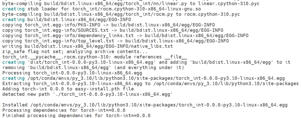
Run python setup.py install to build and install the extension. It should look something like Figure 6:

../../_images/ck-compilation.jpg — Fig. 6 Compilation and installation of the INT8 kernels.#

INT8 model inference and performance#

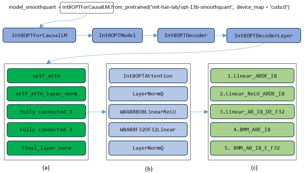
The implementation architecture of running SmoothQuant models on MI300X GPUs is illustrated in Figure 7, where (a) shows the decoder layer composition components of the target model, (b) shows the major implementation class for the decoder layer components, and (c) denotes the underlying GPU kernels implemented by CK instance.

../../_images/ck-inference_flow.jpg — Fig. 7 The implementation architecture of running SmoothQuant models on AMD MI300X accelerators.#

For the target SQ quantized model, each decoder layer contains three major components: attention calculation, layer normalization, and linear transformation in fully connected layers. The corresponding implementation classes for these components are:

Int8OPTAttention
W8A8B8O8LinearReLU
W8A8BF32OF32Linear

These classes’ underlying implementation logits will harness the functions in previous table. Note that for the example, the LayerNormQ module is implemented by the torch native module.

Testing environment: The hardware platform used for testing equips with 256 AMD EPYC 9534 64-Core Processor, 8 AMD Instinct MI300X accelerators and 1.5T memory. The testing was done in a publicly available Docker image from Docker Hub: rocm/pytorch:rocm6.1_ubuntu22.04_py3.10_pytorch_2.1.2

The tested models are OPT-1.3B, 2.7B, 6.7B and 13B FP16 models and the corresponding SmoothQuant INT8 OPT models were obtained from Hugging Face.

Note that since the default values were used for the tunable parameters of the fundamental instance, the performance of the INT8 kernel is suboptimal.

Figure 8 shows the performance comparisons between the original FP16 and the SmoothQuant-quantized INT8 models on a single MI300X accelerator. The GPU memory footprints of SmoothQuant-quantized models are significantly reduced. It also indicates the per-sample inference latency is significantly reduced for all SmoothQuant-quantized OPT models (illustrated in (b)). Notably, the performance of the CK instance-based INT8 kernel steadily improves with an increase in model size.

../../_images/ck-comparisons.jpg — Fig. 8 Performance comparisons between the original FP16 and the SmoothQuant-quantized INT8 models on a single MI300X accelerator.#

For accuracy comparisons between the original FP16 and INT8 models, the evaluation is done by using the first 1,000 samples from the LAMBADA dataset’s validation set. We employ the same Last Token Prediction Accuracy method introduced in SmoothQuant Real-INT8 Inference for PyTorch as our evaluation metric. The comparison results are shown in Table 2.

Table 2 The inference accuracy comparisons of SmoothQuant quantized models on Instinct MI300X.#
Models	Hugging Face FP16 model accuracy	SmoothQuant quantized INT8 model accuracy
opt-1.3B	0.72	0.70
opt-2.7B	0.76	0.75
opt-6.7B	0.80	0.79
opt-13B	0.79	0.77

Conclusion#

CK provides a rich set of template parameters for generating flexible accelerated computing kernels for difference application scenarios.

CK supports multiple instruction sets of AMD Instinct GPUs, operator fusion and different data precisions. Its composability helps users quickly construct operator performance verification.

With CK, you can build more effective AI applications with higher flexibility and better performance on different AMD accelerator platforms.