Using rocprofv2#
Note
rocprofv2 is considered beta software.
rocprofv2 is a command-line interface tool (CLI) that lets you profile AMD GPU applications
without any requirement of source code modification. The usage of rocprofv2 along with
various command-line arguments is described in the following sections.
To see all the rocprofv2 options, refer to rocprofv2 command help, or run the following from the command line:
rocprofv2 --help
Application tracing#
Tracing of application and hardware events, is a primary feature of the rocprofv2 command.
The various options for tracing HIP/HSA API, asynchronous activity, and kernel dispatches
are described in the following table:
Tracing mode |
Option |
Usage |
HIP API tracing |
|
|
Combined HIP API and asynchronous activity tracing |
|
|
HSA API tracing |
|
|
Combined HSA API and asynchronous activity tracing |
|
|
ROCTx API tracing |
|
|
Kernel dispatches tracing |
|
|
All tracing modes combined |
|
|
Note
By default, the output of these options is directed to stdout unless
the -o option is also specified.
To generate output from these trace options, use one of the supported plugins that
generate output in a specific format, as explained in Formatting output using plugins. The default
plugin is the file plugin that generates a CSV file returned to stdout, or
returned to a file when used with -o option.
rocprofv2 supports API tracing at both HIP and HSA level. In general, HIP APIs
directly interact with the user program. It is easier to analyze HIP traces as you
can directly map the traces to the program. HSA API tracing is more suited for
advanced users who want to understand the application behavior at the lower level.
Both HIP and HSA APIs support asynchronous behavior (e.g., asynchronous
memory copy). If trace collection is triggered using either --hip-api
or --hsa-api, the trace records only the start, stop, and duration of
API events, but not the execution time of associated actions like memory copy.
To record the duration of asynchronous activities, use --hip-activity and
--hsa-activity options, which record both the API events and asynchronous
events.
Visualize tracing results#
You can view the traces generated by rocprofv2 using the Perfetto UI that
enables you to view and analyze traces in a web browser. To begin go to
Perfetto UI, select Open trace file
from the left-side menu, and select the ROCProfiler trace file to view.
The following is a screenshot from the Perfetto interface. The tasks are organized in a Gantt chart style with the x-axis representing time and each rectangle representing the start and the end time of a task. The tasks are organized in rows. In the figure is the HIP API, HSA API, a queue, and a stream.
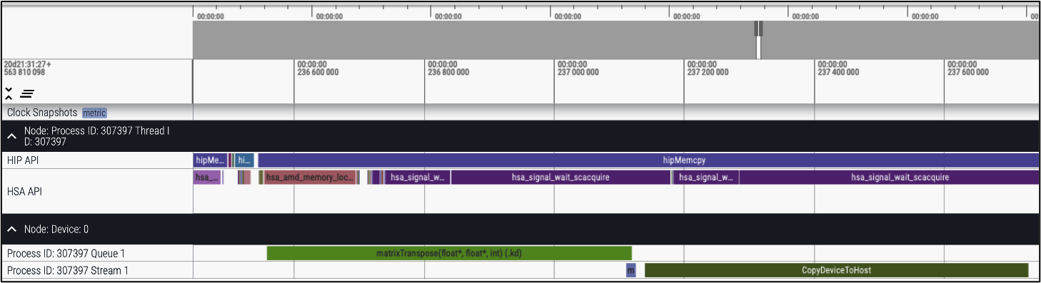
Fig. 9 Visualizing Traces Generated Using sys-trace#
Tip
To enlarge the image, right click on the image and use the Open image in new tab option.
Kernel profiling#
As explained in rocprof-counters application tracing lets you evaluate the timeline of application events, but is little help in providing insight into kernel execution details. The kernel profiling functionality lets you select kernels for profiling and choose the basic counters or derived metrics to be collected for each kernel execution, thus providing a greater insight into hardware performance.
To check the supported performance counters and metrics, use:
rocprofv2 --list-counters
The following is a sample output from the --list-counters option. The output has
been truncated for explanation:
gfx1030:0 : SQ_WAVES
: Count number of waves sent to SQs. {emulated, global, C1}
block SQ can only handle 8 counters at a time
The fields in the output are:
gfx1030:0 - The GPU architecture and GPU ID (separated by colon). The GPU ID needs to be specified as there might be multiple GPUs in the system.
SQ_WAVES - The counter name. Typically, the first token before the first underscore is the GPU block name. Here, SQ is the block that is responsible for managing wavefronts and issuing instructions.
Note
For more information on the performance counters available on AMD GPUs, refer to the GPU architecture documentation.
Input file#
To collect basic counters and derived metrics, define the profiling scope in an input file, and specify the file on the command line:
rocprofv2 -i input.txt <app_relative_path>
An input file is a text file that can be supplied to rocprofv2 for basic
counter and derived metric collection. It contains the list of basic counters or derived metrics to be collected.
Sample Input File:
pmc: SQ_WAVES TA_UTIL
The fields in the input file are detailed in Input File.
PMC: The rows in the text file beginning with pmc: are the group of
basic counters or derived metrics the user is interested in collecting.
The basic counters or derived metrics can be selected from the output
generated by --list-counters option.
The number of basic counters or derived metrics that can be collected in
one run of profiling is limited by the GPU hardware resources. If too
many counters/metrics are selected, the kernels need to be executed
multiple times to collect the counters/metrics. For multi-pass
execution, include multiple rows of pmc: in the input file. Counters or
metrics in each pmc: row can be collected in each run of the kernel.
GPU: The row beginning with the keyword gpu: specifies the GPU(s) on
which the hardware counters are to be collected. This enables the
support for profiling multiple GPUs. You can specify multiple GPUs
separated by comma such as gpu: 1,3.
Kernel: The row beginning with the kernel: keyword specifies the
names of kernels to be profiled.
Range: The row beginning with the keyword range: specifies the range
of kernel dispatches. Specifying range is helpful in cases where the
application causes multiple kernel dispatches and users want to filter
some kernel dispatches. In the above example, the range: 0:1 depicts that
one kernel is profiled.
Kernel profiling output#
This section discusses the kernel profiling output generated using the
Input File. rocprofv2 reports one value per metric per
kernel in the output. You can generate the output in desired format
as described in Formatting output using plugins. If no plugin is
specified while generating the output, the result is dumped on the
command-line.
The following sample output is generated using the file plugin. Each
row of the file is an instance of kernel execution.
For each kernel, basic information (e.g., GPU_ID, SGPR, PID, etc.) and
performance counters (specified in the input file) values are listed.
The information is generated in the format of field name and value.
$ rocprofv2 -i input.txt --plugin file -o result MatrixTranspose

$ cat results_result.csv

Dispatch_ID,GPU_ID,Queue_ID,Queue_Index,PID,TID,GRD,WGR,LDS,SCR,Arch_VGPR,ACCUM_VGPR,
SGPR,Wave_Size,SIG,OBJ,Kernel_Name,Start_Timestamp,End_Timestamp,Correlation_ID,
SQ_WAVES,GRBM_COUNT,GRBM_GUI_ACTIVE,SQ_INSTS_VALU,FETCH_SIZE

1,64700,1,0,353,353,1048576,16,0,0,8,0,16,64,140356026185088,1,"matrixTranspose(float*, float*, int)
(.kd)",7,30064771072,0,65536.000000,398333.000000,398333.000000,917504.000000,4136.000000

2,64700,1,2,353,353,1048576,16,0,0,8,0,16,64,140356026184832,2,"matrixTranspose(float*,
float*, int)
(.kd)",7,30064771072,0,65536.000000,586424.000000,586424.000000,917504.000000,4130.437500

3,64700,1,4,353,353,1048576,16,0,0,8,0,16,64,140356026184576,3,"matrixTranspose(float*,
float*, int)
(.kd)",7,30064771072,0,65536.000000,392460.000000,392460.000000,917504.000000,4129.937500
The fields in the output file are:
Output fields |
Description |
|---|---|
|
Kernel’s dispatch Id |
|
GPU identifier to which the kernel was submitted |
|
ROCm queue unique identifier to which the kernel was submitted |
|
ROCm queue write index for the submitted AQL packet |
|
System application process id that submitted the kernel |
|
System application thread id that submitted the kernel |
|
Kernel’s grid size |
|
Kernel’s work group size |
|
Kernel’s Local Data Share (LDS) memory size |
|
Kernel’s scratch memory size |
|
Number of Vector General Purpose Registers (VGPR) used in kernel dispatch |
|
Total Count of VGPRs |
|
Kernel’s Scalar General-Purpose Register (SGPR) size |
|
Number of wavefronts |
|
Kernel’s completion signal |
|
Code object |
|
Name of the dispatched kernel |
|
Begin time in nanoseconds (ns) when the kernel begins execution |
|
End time in ns when the kernel finishes execution |
|
Unique identifier for correlation between HIP and HSA async calls during activity tracing |
You can view the generated output using the Perfetto UI as previously described in Visualize Tracing Results. The following is a screenshot of the Perfetto UI when viewing the kernel profiling output.
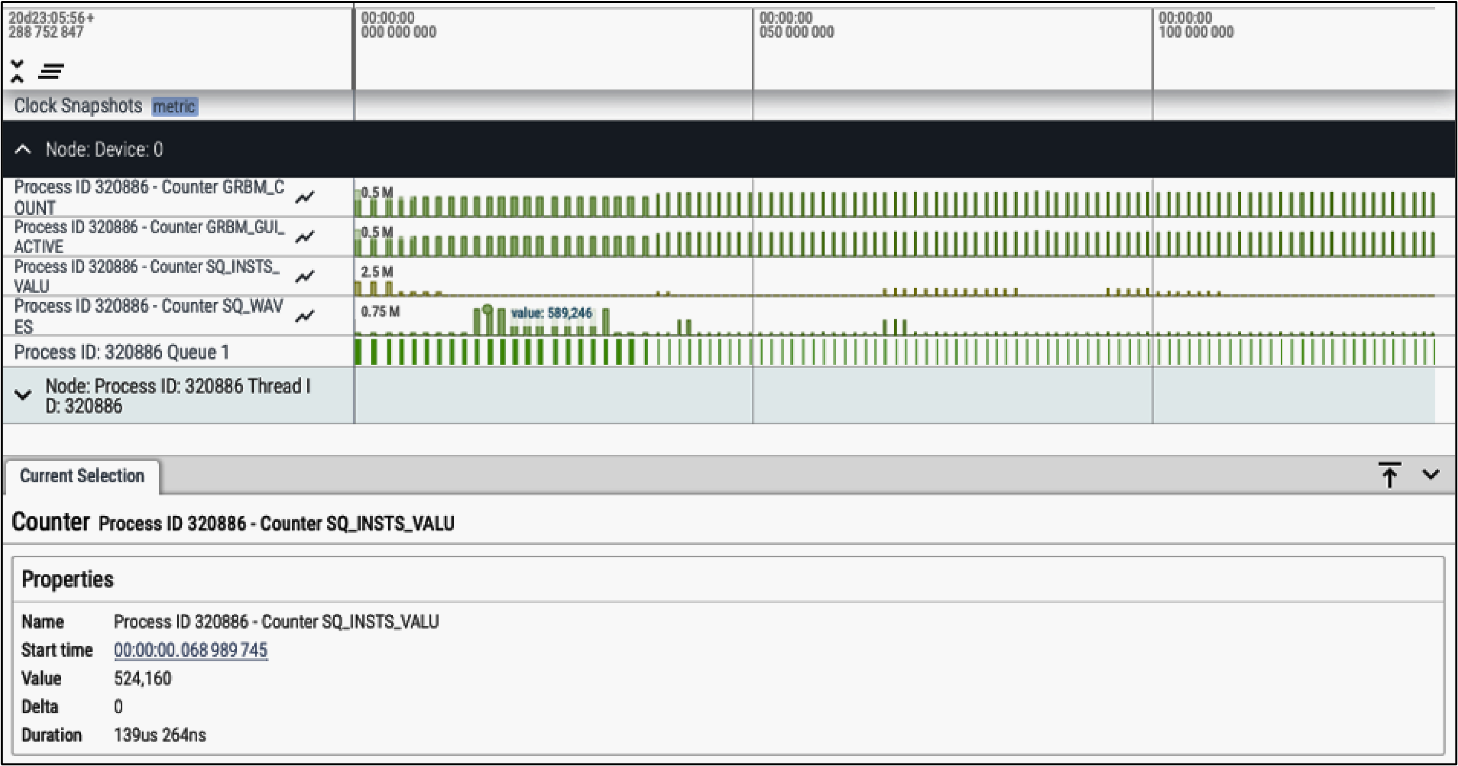
Fig. 10 Viewing kernel profiling output#
The first four rows represent the performance counters as
specified in the input file. The last row is the kernel execution
timeline, which is the same as the --kernel-trace option used in the
Application tracing mode.
Viewing the profile results provides a good overview of kernel execution times and how performance metrics values change across the kernels. Additionally, you can also see the exact value of a counter/metric by hovering over or clicking the bar.
Formatting output using plugins#
rocprofv2 uses a modular plugin system which allows you to generate
profiling output in the desired format. Because these plugins are modular in
nature, they can easily be decoupled from the code based on need. By
default, rocprofv2 generates the profiling output using the file and CLI
plugins.
You can install other plugins (as listed in the table below) using the plugins package as shown:
rocprofiler-plugins_2.0.0-local_amd64.deb
-or-
rocprofiler-plugins-2.0.0-local.x86_64.rpm
You can also create your own plugins if you are using rocprofv2 with source code and not just as a CLI tool. To write new plugins import the include/rocprofiler/v2/rocprofiler_plugins.h header file.
To generate the profiling output using a plugin, use:
rocprofv2 --plugin plugin_name -i input.txt <app_relative_path>

# where plugin_name is file, perfetto, or ctf
To specify the plugin version to be used in case of multiple versions, use:
rocprofv2 --plugin <plugin_name> --plugin-version <plugin_version_required> <rocprofv2_options> <app_relative_path>
The following table lists the available plugins:
Plugin |
Output format |
|---|---|
File |
Text files (.csv or .txt) |
Perfetto |
Protobuf in the format of the Chromium Project’s trace-event format |
Common Trace Format (CTF) |
Binary, formatted in the ctf format that can be consumed by public tools such as Babeltrace and TraceCompass |
Note
To generate output, the plugins require you to set the OUTPUT_PATH variable to the desired directory. File plugin is the only plugin that still generates output in the absence of OUTPUT_PATH by dumping the output to standard output.
File plugin#
To output the data in .txt files using file plugin, use:
rocprofv2 --plugin file -i samples/input.txt -d output_dir <app_relative_path>
Note that specifying the directory for output files using -d is optional.
File plugin has two versions with version 2 being the default. The headers in the output files generated using file plugin version 1 and 2 differ as shown below.
Version 1 header:
Index,KernelName,gpu-id,queue-id,queue-index,pid,tid,grd,wgr,lds,scr,arch_vgpr,accum_vgpr,sgpr,wave_size,sig,obj,DispatchNs,BeginNs,EndNs,CompleteNs,Counters
Note that the version 1 header is same as the legacy rocprof output.
Version 2 header:
Dispatch_ID,GPU_ID,Queue_ID,PID,TID,Grid_Size,Workgroup_Size,LDS_Per_Workgroup,Scratch_Per_Workitem,Arch_VGPR,Accum_VGPR,SGPR,Wave_Size,Kernel_Name,Start_Timestamp,End_Timestamp,Correlation_ID,Counters
Perfetto plugin#
To output the data in Protobuf format using the Perfetto plugin, use:
rocprofv2 --plugin perfetto --hsa-trace <app_relative_path>
You can view the Protobuf files using Perfetto or Trace processor.
Common Trace Format plugin#
To output the data in Common Trace Format (CTF), which is a binary trace format, use:
rocprofv2 --plugin ctf --hip-trace <app_relative_path>
You can view the CTF binary output using TraceCompass or Babeltrace.