Visualize and analyze GPU thread trace data#
2026-06-22
11 min read time
ROCprof Compute Viewer interprets the output of ui_output_agent_{agent_id}_dispatch_{dispatch_id} file for visualization. The visualization includes:
Source visualization (go to Trace -> ISA)
Hotspot analysis
Memory ops to
waitcntdependencyOccupancy visualization
Flamegraph view (per-target-CU/SIMD source/ISA stack rollup, plus a global marker flamegraph when SQTT instrumentation is present)
SQTT instrumentation marker visualization (from the
.sqtt_funcmapELF section emitted by the LLVM pass)
RCV accepts two kinds of input:
A
rocprofv3UI output directory (JSON), produced whenrocprofv3converts the thread trace for you.A directory of raw
.att/.outthread-trace files captured directly through the rocprofiler-sdk API. These require a decoder-enabled build.
To launch the Compute Viewer with a rocprofv3 UI output directory, use any of the following methods:
Go to Menu -> Import -> Rocprofv3 UI Output
Provide the full path to “Ui path”
Use command line:
./rcviewer <dir_to_ui_folder>
To open raw .att/.out files directly (decoder-enabled build):
Go to Menu -> Import -> ATT Trace Files… and select the
.att/.outfiles.Or pass the directory on the command line:
./rcviewer <dir_with_att_out_files>
When the raw trace was captured via the rocprofiler-sdk API it has no code.json/snapshots.json, so the Instructions view and source pane stay empty until you regenerate that correlation from the kernel code objects:
python3 scripts/generate_snapshot.py kernel_code_object_id_1.out kernel_code_object_id_2.out
This writes code.json, snapshots.json, and copies of the referenced source files into the current directory, which you then pass to the viewer.
The various views available as tabs on the top are described in the following sections.
Requirements#
To ensure that rocprofv3 generates the thread trace data correctly, install the following components:
AQL profile:
Available with ROCm 7.0 or later, or build from source.
If
rocprofv3throws INVALID_SHADER_DATA error, the AQL profile and Trace Decoder versions are incompatible.
ROCprofiler-SDK:
Available with ROCm 7.0 or later, or build from source.
ROCprof Trace Decoder:
Bundled with
rocprofv3since ROCm 7.13, so no extra install is needed. On ROCm versions earlier than 7.13, build from source.
For instructions on how to run rocprofv3 to collect thread trace data, see using rocprofv3 to collect thread trace.
Hotspot view#
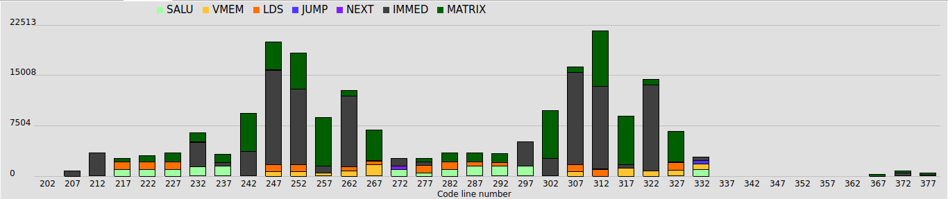
The Hotspot tab displays a histogram of instruction costs.
Vertical axis (Cycles): Total accumulated latency cycles for each bin based on the bin’s center value.
To adjust the number of bins and histogram range, go to Edit -> Hotspot Options. Clicking a bin highlights the first and last ISA lines present in the bin.
The hotspot is computed over all waves within the “WaveView Clock Range”.
IMMED instructions such as
s_nop,s_waitcnt, ands_barriermight appear to over-represent cycles since waves in a SIMD often wait concurrently.IDLE time is not computed into hotspot; only EXECUTE and STALL.
Compute Unit and Utilization view#
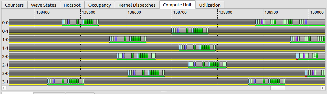
The Compute Unit tab displays the trace aggregated per wave. The trace is separated per SIMD-Slot such as “2-6”.
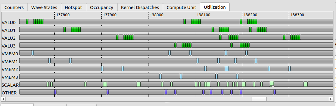
The Utilization tab displays the trace aggregated per SIMD. The trace is separated per instruction type such as VALU, VMEM, SCALAR, and OTHER. This view hides IMMED type tokens as multiple waves could be executing them in parallel. The Utilization view displays only ISSUE for gfx or EXECUTION for gfx10+ and hides STALLED time. This view can be used to identify bubbles. Note that in case of overlapping tokens from different wave slots, only one token is displayed.
Here are the user controls for Compute Unit and Utilization views:
Right-click and drag to measure number of cycles.
Left-click highlights the ISA corresponding to that token.
If no ISA is highlighted, it is likely that the token couldn’t be matched with the ISA. Check for warnings on the
rocprofv3output.
Use A and D keys for panning.
Use Shift + MouseWheel to scroll the timeline horizontally.
Use WaveView zoom box on the left panel or CTRL + MouseWheel to control the zoom level.
Instructions view#
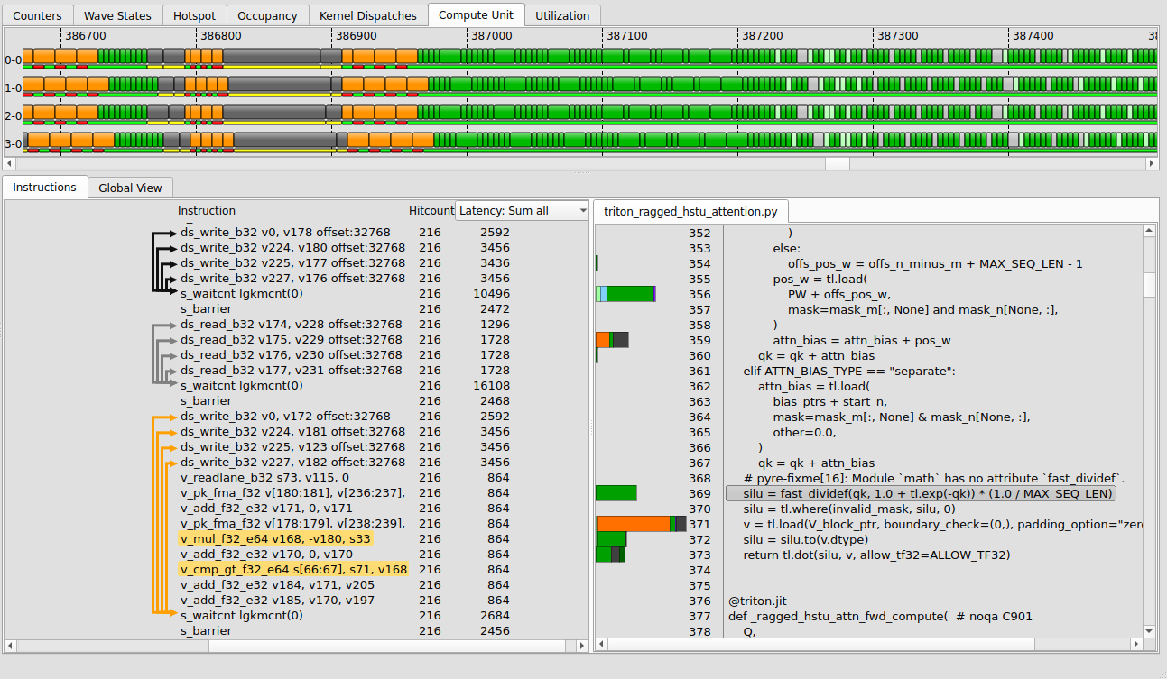
The ISA view is available under Compute Unit and Utilization tabs. The ISA view consists of a list of instructions along with their “Hitcount” and “Latency” cost. If debug symbols are present, rocprofv3 snapshots the related source files, as shown on the right side of the image.
The cost can be calculated as a mean or sum of the selected wave, mean or sum of all waves, or display a particular loop iteration.
Arrows link memory operations to the
s_waitcntwaiting on them. This instruction view is per wave. Another wave that takes a different execution path might present a different set of arrows or links.Clicking on the instruction scrolls the trace bar in the Compute Unit and Utilization views to the cycle corresponding to the instruction execution, with left alignment.
Left click on a token highlights the ISA line corresponding to that instruction.
Hover or click on an ISA line to highlight the corresponding source line, as seen on the right-hand side of the image. Vice versa is also applicable.
Clicking on a source line keeps the corresponding ISA line highlighted until you click on the same or another line.
Global view#
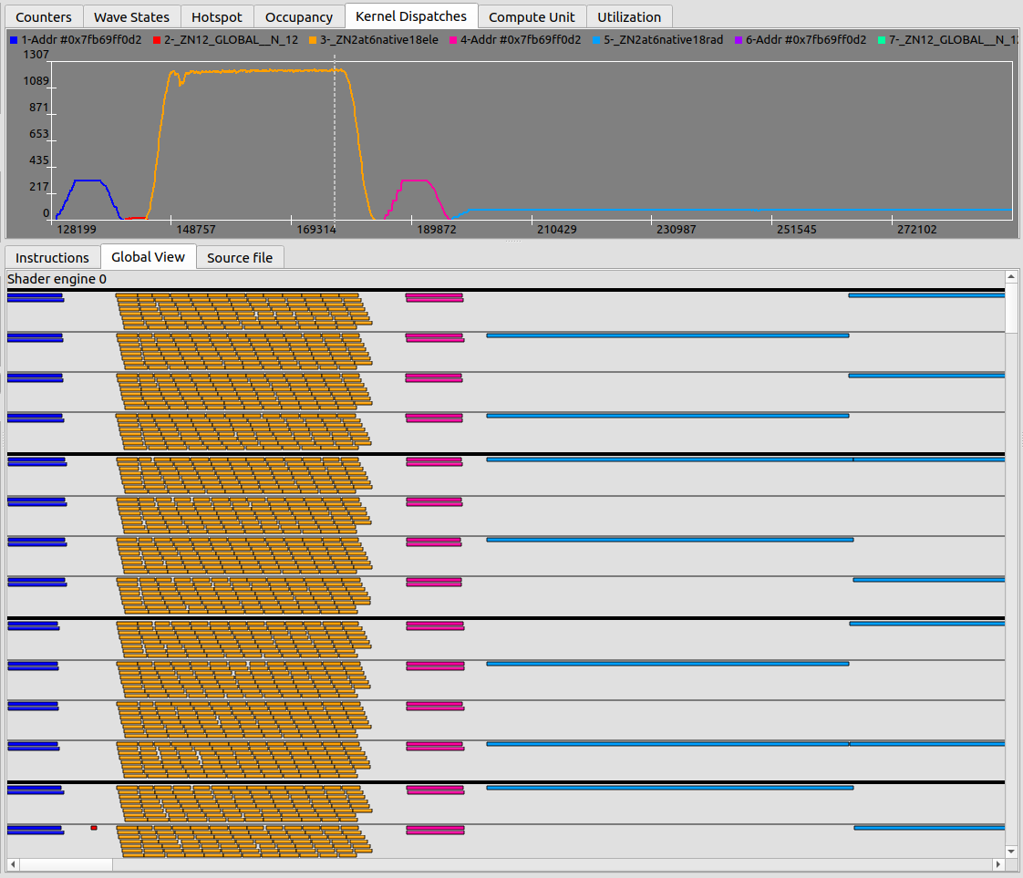
The Global View tab presents a comprehensive trace of all waves across the enabled SEs, with each wave color-coded according to the kernel.
Hovering over the trace displays additional information, such as the kernel being run by the wave, the CU or SIMD or slot, and wave duration.
The Global view can be compared with the Kernel dispatch plot.
Right-click and drag to measure number of cycles.
Summary view#
The Summary tab is available with AMD Instinct MI200 and MI300 series accelerators. It displays the following information:
Average instruction cost for the whole trace according to the state IDLE, ISSUE, and STALL.
Average hardware utilization according to the instruction type VALU, VMEM, LDS, and so on.
Per-compute hardware utilization values and accumulated counters.
To enable the summary view, use the following parameters:
# SQ_ACTIVE_INST_X collects activity for token type X.
# For summary, a collection interval of 10 is enough.

rocprofv3 --att-perfcounter-ctrl 10 --att-perfcounters "SQ_BUSY_CU_CYCLES SQ_VALU_MFMA_BUSY_CYCLES SQ_ACTIVE_INST_VALU SQ_ACTIVE_INST_LDS SQ_ACTIVE_INST_VMEM SQ_ACTIVE_INST_FLAT SQ_ACTIVE_INST_SCA SQ_ACTIVE_INST_MISC"

# Or using the convenience parameter

rocprofv3 --att-activity 10
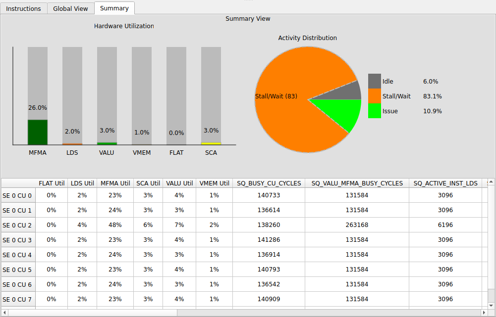
Per-CU rates are averaged over the period in which any wave was present in the CU.
Peak rate indicates the maximum across any given cycle, calculated by summing all SEs and CUs.
Utilization for counter X is computed as:
For peak rates: \(max_over_cycles(add_over_cu(X))/max_over_cycles(add_over_cu(SQ_BUSY_CU_CYCLES))\)
For other values: \(add_all(X)/add_all(SQ_BUSY_CU_CYCLES)\)
Occupancy and Kernel dispatch views#
Here are the user controls for Occupancy and Kernel dispatch views:
Use the mouse wheel to zoom plots in and out.
Pressing Left CTRL button zooms in and out on the vertical axis.
Click and drag to select an area.
Right-click and drag for panning.
Clicking on a token in the waveview (trace) adds a blue marker to identify the cycle for that token.
Note
The standalone Wave States tab (a vertical slice of the Compute Unit view showing the number of active waves in each state: IDLE, EXEC, STALL, and WAIT) has been temporarily removed. Its functionality will eventually be absorbed into the Counters view. The wave-state coloring within the Compute Unit view itself is unaffected.
Occupancy view#
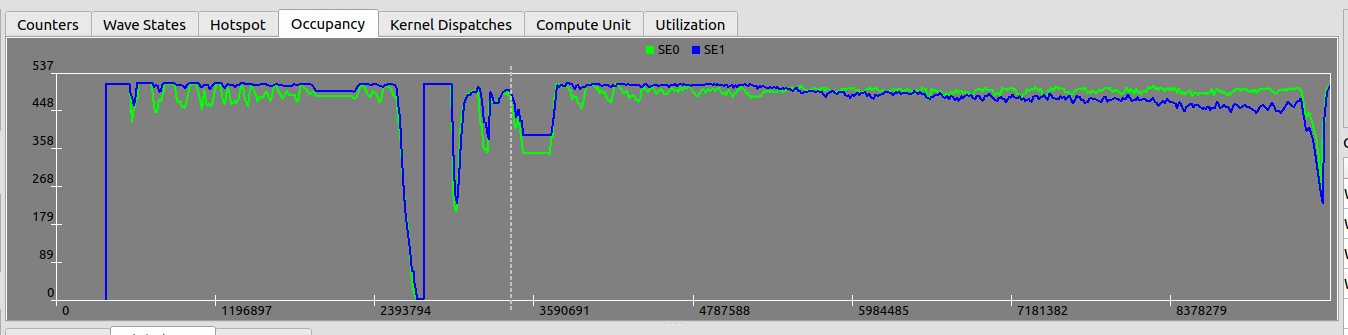
The Occupancy tab shows occupancy per Shader Engine (SE) as a number of waves.
Kernel dispatch view#
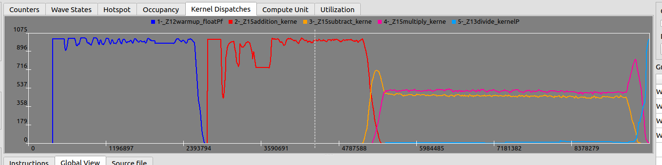
The Kernel Dispatches tab shows occupancy per kernel. This tab is usually relevant when there are multiple kernels running on different streams.
Settings#
The left panel contains settings that help you configure the Compute Viewer.
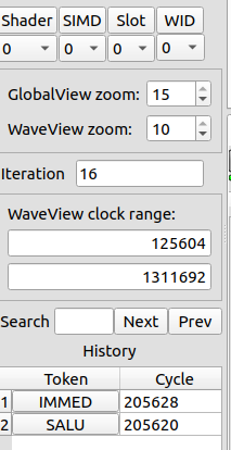
The settings as shown in the preceding image are explained here:
The Shader (Shader Engine), SIMD, Slot (Wave slot within a SIMD), and WID (A wave ID counter for that slot) boxes allow you to select the target wave.
The operations in the Instruction tab such as Token-to-ISA mapping, loop iteration navigation, and so on, are performed only on the selected target wave.
The WaveView Clock range box defines the visible cycles in the Compute Unit and Utilization tabs. It’s also used in the hotspot calculation.
By default, set the range from the first cycle to a little after the last cycle of the target wave.
Reduce the start and end range to make navigation easier.
Increase start and end range to see more waves or get a more general hotspot calculation.
The GlobalView Zoom box defines the zoom level for the GlobalView tab. Value range: [0,15].
The WaveView zoom box defines the zoom level for the wave view or trace. Value range: [0,10].
The Iteration box defines the iteration for the selected token.
Left click on a token to update the iteration.
This value can be edited by scrolling the view to the same instruction on a different loop iteration.
Makes navigating loops easier.
The iteration is defined as the number of times a specific instruction is executed for each wave (starting at zero).
The Search box searches for a specific text in the instruction view. For example, search for
ds_to find the first LDS instruction.The History box contains the history (token + cycle) of previously selected tokens. It can be used to go back to a previous location.
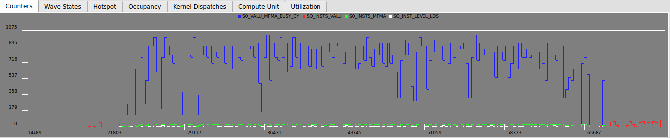
Counters view#
The Counters tab displays a plot of SQ counter collection in a given period. You can add up to eight counters, while it’s recommended to add four. With AMD Instinct MI300, --att-perfcounter-ctrl 3 has a polling rate of 120~240 cycles.
To Stream SQ performance counters to the thread trace buffer in the given relative period, use:
rocprofv3 --att-perfcounter-ctrl 3 --att-perfcounters "SQ_VALU_MFMA_BUSY_CYCLES SQ_INSTS_VALU SQ_INSTS_MFMA SQ_INST_LEVEL_LDS"
To stream SQ performance counters for all or specific SIMDs, define SIMD masks using :0xmask in which the counters increment only for a particular SIMD. The default value of 0xF increments counters for all SIMDs.
# This enables SQ_INSTS_VALU for all SIMDs, and shows individual SQ_INSTS_SALU counters per SIMD [0,1,2]
rocprofv3 --att-perfcounter-ctrl 3 --att-perfcounters "SQ_INSTS_VALU:0xF SQ_INSTS_SALU:0x1 SQ_INSTS_SALU:0x2 SQ_INSTS_SALU:0x4"
To view the plot for SQ counters collected per Compute Unit (CU) or SE:
Go to Menu -> Edit -> Counters shown to define the SE or CU to be plotted.
Deselect all CUs except “1” to visualize counters only for CU=1. Note that “1” is usually the default
--att-target-cu.
To view the plot for SQ counters collected per SIMD, use SIMD mask and filter the CU in “Menu -> Edit -> Counters shown”.
On ROCm 7.13 or later, collect counters only for the target CU with --att-perfcounter-target-only. This is recommended when using a high polling rate:
rocprofv3 --att-perfcounter-target-only 1 [...]
Here are the SQ counters that help to analyze hardware utilization:
SQ_INST_LEVEL_LDS - Measures the current number of in-flight LDS instructions.
SQ_VALU_MFMA_BUSY_CYCLES - Measures the current MFMA hardware utilization.
The following figure shows the MFMA, VALU, and LDS counters. MFMA_BUSY_CYCLES and INST_LEVEL_LDS count current pipeline activity, while SQ_INSTS_VALU and SQ_INSTS_MFMA count the number of instructions issued.
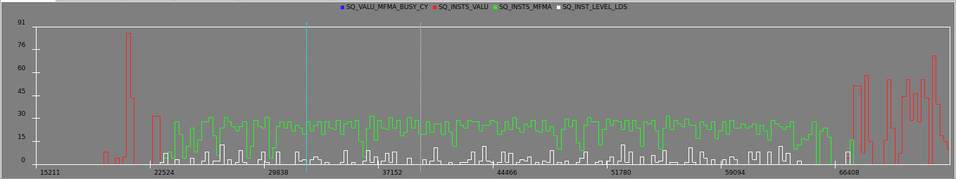
Here is a zoomed-in view of the preceding figure.
Derived counters#
In addition to the raw SQ counters, RCV lets you define derived counters that are evaluated in real time. Go to Menu -> Edit -> Derived Counters.
Some simple derived counters are provided by default, such as
MFMA_util,VALU_util, andLDS_util.Use the “Help” button to see the derived counter syntax.
Create, delete, and edit user-defined derived counters.
If multiple files are present, the currently selected widget tab defines which derived counter list is shown.
The left list shows the raw (basic) counters collected with SQTT, along with their shapes (XCC, SE, CU, Time).
Flamegraph view#
The Flamegraph view (which replaces the previous Explorer view) rolls up latency into a stack so you can quickly find the most expensive code paths.
Frames are sized by accumulated latency cycles; wider frames cost more.
The stack is built per target CU/SIMD over the source and ISA, so you can drill from a source line down to the individual instructions.
Hover a frame to see its latency; click to zoom into that frame.
When the trace contains SQTT instrumentation markers, a separate global marker flamegraph is also available, rolling up time spent inside instrumented regions.
Troubleshooting#
Issue: RCV doesn’t display anything except “Occupancy” and the stats_*.csv file is empty.
Solution: Thread trace receives detailed information from the target_cu. If the application doesn’t populate the target_cu, then nothing will be traced.
For possible solutions, see thread trace documentation.