HIP Graph API Tutorial

Time to complete: 60 minutes | Difficulty: Intermediate | Domain: Medical Imaging

Introduction

Imagine you are directing a movie. In traditional GPU programming with streams, you are like a director who must call “action!” for every single shot, waiting between each take. With HIP graphs, you pre-plan the entire scene sequence and then call “action!” just once to film everything in one go. This tutorial will show you how to transform your GPU applications from repeated direction to choreographed performance.

Modeling dependencies between GPU operations

Most movies in the world follow a plot where certain scenes must happen before the following scenes; otherwise the movie might not make much sense. If a scene A must happen before scenes B and C, B and C depend on A. If B and C contain different stories that (at this point) are unrelated to each other, B and C are independent and can be shown to the audience in any order. However, both scenes might be a prerequisite for the final scene D, so D depends on both of them. When you represent scenes as nodes and dependencies as edges, you can create a graph, and the graph representing your imaginary movie script will have a diamond-like shape:

You can think about GPU operations in a similar way. For example, most kernels require at least one data buffer to work with, so they will depend on a preceding copy or memset operation. Others might process the results of preceding kernels. Real-world applications typically involve multiple GPU operations with dependencies between them. HIP offers two ways to think about and model these dependencies: streams and graphs.

Streams

Streams are HIP’s default model for organizing and launching GPU operations on the device. They are sequential sets of operations, similar to CPU threads. Adding operation A before operation B to a stream ensures A happens before B, regardless of any interdependencies (or lack thereof) between them. A stream can be thought of as a first-in, first-out (FIFO) queue of operations.

Multiple streams operate independently, and manual synchronization is required when dependencies cross stream boundaries. Additionally, each operation in a stream is scheduled independently, which — depending on the complexity of the enqueued operation — might lead to noticeable CPU launch overhead and kernel dispatch latency, especially for workloads with many small kernels. However, applications that use streams are well suited for workloads that are dynamic and unpredictable.

For more information about HIP streams, see Asynchronous concurrent execution.

Graphs

HIP graphs model dependencies between operations as nodes and edges on a diagram. Each node in the graph represents an operation, and each edge represents a dependency between two nodes. If no edge exists between two nodes, they are independent and can execute in any order.

Because dependency information is built into the graph, the HIP runtime automatically inserts the necessary synchronization points. Launching all operations in a graph requires only a single API call, reducing launch overhead and dispatch latency to near-zero. This is especially beneficial for workloads with many small kernels, where launch overhead can dominate overall execution time.

Graphs must be defined once before use, making them ideal for fixed workflows that run repeatedly. While node parameters can be updated between executions, the graph structure itself cannot change after instantiation. This structural immutability is the primary trade-off compared to the flexibility of streams.

For more information about HIP graphs, see HIP graphs.

When to use graphs

This table shows when to use graphs in your application.

✅ Use Graphs When	❌ Avoid Graphs When
Workflow is fixed and repetitive	Workflow changes dynamically
Same kernels execute many times	One-shot operations
Launch overhead is significant (many small kernels)	Kernels are long-running

Transitioning a CT reconstruction pipeline

In this tutorial, you will modify an existing GPU-accelerated stream-based image processing pipeline that reconstructs computer tomography (CT) data (the classic Shepp-Logan phantom [ShLo74]). The pipeline transforms raw X-ray projections into clear cross-sectional images used in medical diagnosis.

Note

The tutorial application generates a phantom volume and forward projections. This GPU-accelerated operation uses multiple streams and appears in the traces. You can ignore the dataset generation — it is not relevant to this tutorial.

The reconstruction pipeline consists of:

1. Load projection data into GPU memory

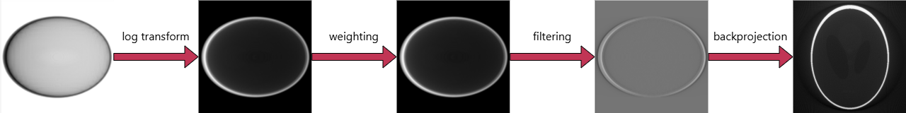
2. Preprocess the projection through six stages:

1. Logarithmic transformation (convert X-ray intensities)

2. Pixel weighting (correct for cone-beam geometry)

3. Forward FFT (transform to frequency domain)

4. Shepp-Logan filtering (enhance edges and improve contrast)

5. Inverse FFT (return to spatial domain)

6. Normalization (account for unnormalized FFT)

3. Reconstruct the 3D volume using the Feldkamp-Davis-Kress (FDK) algorithm [FeDK84]

Why HIP graphs? CT scanners process hundreds of projections per scan. By capturing this fixed workflow as a graph, you will reduce the amount of API calls required for launching the workflow on a GPU to 1 per projection, thus reducing launch overhead and dispatch latency to near-zero.

What you will learn

After completing this tutorial, you will be able to:

• Convert a stream-based HIP application to a graph-based application via stream capturing

• Create graphs manually for fine-grained control

• Integrate graph-safe libraries like hipFFT into your graphs

• Understand when graphs provide performance benefits

• Apply graph concepts to your own workflows

Before you begin

Required knowledge

You should be comfortable writing and debugging HIP kernels, understand basic GPU memory management concepts like device allocation and host-to-device transfers, be familiar with HIP streams and events, and have experience using CMake to build C++ projects. This tutorial assumes you have written at least a few HIP programs before and understand concepts like grid dimensions and thread blocks.

Hardware and software requirements

Your system needs ROCm 6.2 or later with the hipFFT library installed. The tutorial works on all supported AMD GPUs, though at least 4 GiB of GPU memory are recommended for comfortable performance with the reconstruction workload. You will also need git to check out the code repository, CMake 3.21 or later to build the code, along with a CMake generator that supports the HIP language such as GNU Make or Ninja.

Note

Visual Studio generators currently do not support HIP. The (optional) rocprofv3 tool is currently supported on Linux only.

To save the output volume, you need a recent version of libTIFF. If CMake cannot find libTIFF on your system, it automatically downloads and builds it.

To view both the input projections and the output volume produced by this tutorial, install a scientific image viewer that can display 16-bit and 32-bit grayscale data, such as Fiji. Standard image viewers may be unable to correctly display the output.

Optional knowledge

While not required, familiarity with Fast Fourier Transform (FFT) operations will help you understand the filtering steps. Similarly, knowledge of medical imaging or CT reconstruction is helpful for understanding the application context. If you have worked with signal processing or image filtering before, you will recognize some of the applied concepts.

Note

You can skip the reconstruction algorithm and concentrate on the stream and graph implementations in the files prefixed with main_.

Step 1: Build the tutorial code

The full code for this tutorial is part of the ROCm examples repository. Check out the repository:

git clone https://github.com/ROCm/rocm-examples.git

Then navigate to rocm-examples/HIP-Doc/Tutorials/graph_api/. The code can be found in the src subdirectory.

Create a separate build directory inside rocm-examples/HIP-Doc/Tutorials/graph_api/. Then configure the project (adjust CMAKE_HIP_ARCHITECTURES to match your GPU):

cd build
cmake -DCMAKE_PREFIX_PATH=/opt/rocm -DCMAKE_BUILD_TYPE=Release -DCMAKE_HIP_ARCHITECTURES=gfx1100 -DCMAKE_HIP_PLATFORM=amd -DCMAKE_CXX_COMPILER=amdclang++ -DCMAKE_C_COMPILER=amdclang -DCMAKE_HIP_COMPILER=amdclang++ ..

Now you can build the three variants of the tutorial code:

cmake --build . --target hip_graph_api_tutorial_streams hip_graph_api_tutorial_graph_capture hip_graph_api_tutorial_graph_creation

Note

The graph_capture variant is currently not supported on Windows and the build target is therefore unavailable.

Step 2: Examining the stream-based baseline application

Open src/main_streams.hip in your editor. You will explore how this application processes data.

Understanding batched processing

The application processes multiple projections simultaneously to maximize GPU utilization.

Determining parallel capacity

At the beginning of main(), the program queries the GPU for its number of asynchronous engines to determine how many streams it can create, indicating how many data transfer or compute operations can run in parallel.

// Fetch device properties
auto devProps = hipDeviceProp_t{};
hip_check(hipGetDeviceProperties(&devProps, 0));

auto const numStreams = devProps.asyncEngineCount;

std::cout << "Device has " << numStreams << " asynchronous engines; preprocessing will use "
          << numStreams << " parallel streams." << std::endl;

auto streams = std::vector<hipStream_t>{};
streams.resize(numStreams);
for(auto&& stream : streams)
    hip_check(hipStreamCreate(&stream));

Tip

Each asynchronous engine executes operations independently. More engines mean more parallelism.

Processing projections in batches

Find the MAIN LOOP comment. Here the application groups projections into parallel batches:

auto projIdx = 0;
while(projIdx < projGeom.numProj)
{
    auto batchSize = std::min(numStreams, static_cast<int>(projGeom.numProj - projIdx));

    // Launch batch in parallel streams
    for(auto streamIdx = 0; streamIdx < batchSize; ++streamIdx, ++projIdx)
    {
        auto stream = streams.at(streamIdx);

Notice how each batch size equals the stream count — this ensures every stream stays busy.

Synchronization

Each projection processes independently, so you only need to synchronize once at the end. hipStreamWaitEvent() function makes the first stream wait for all other streams to complete.

// First stream waits for other streams to complete
auto completionEvents = std::vector<hipEvent_t>{};
for(auto streamIdx = 1; streamIdx < streams.size(); ++streamIdx)
{
    auto event = hipEvent_t{};
    hip_check(hipEventCreate(&event));
    hip_check(hipEventRecord(event, streams.at(streamIdx)));
    completionEvents.push_back(event);
}

for(auto&& event : completionEvents)
    hip_check(hipStreamWaitEvent(streams.at(0), event));

Exploring the processing pipeline

Next, examine what happens to each projection. Find the START HERE comment to see the reconstruction pipeline’s first steps:

////////////////////////////////////////////////////////////////////////////////////////////////////
// START HERE
////////////////////////////////////////////////////////////////////////////////////////////////////
auto proj = projections.at(streamIdx);
auto projPitch = projectionPitches.at(streamIdx);
normalization_kernel<<<blocksPerGrid, threadsPerBlock, 0, stream>>>(
    input, inputPitch, proj, projPitch, projGeom.dim, projGeom.bps
);

log_transformation_kernel<<<blocksPerGrid, threadsPerBlock, 0, stream>>>(proj, projPitch, projGeom.dim);

weighting_kernel<<<blocksPerGrid, threadsPerBlock, 0, stream>>>(
    proj,
    projPitch,
    projGeom.dim,
    projGeom.d_sd,
    projGeom.d_so,
    projGeom.minCoord,
    projGeom.pixelDim
);

This is a typical pattern found across many HIP applications: multiple kernels executing in sequence with data dependencies. In the next step, the weighted projections need to be transformed into Fourier space and filtered. For optimal performance, it is recommended to execute a 1D FFT on a buffer size which is a power of two. Copy the weighted projection to another buffer where the row length is a power of two equal to or larger than the projection’s row length:

// Expand projection to filter length
auto expanded = expandedProjections.at(streamIdx);
auto expandedPitch = expandedPitches.at(streamIdx);
hip_check(hipMemset2DAsync(
    expanded, expandedPitch, 0, projGeom.dimFFT.x * sizeof(float), projGeom.dimFFT.y, stream
));
hip_check(hipMemcpy2DAsync(
    expanded,
    expandedPitch,
    proj,
    projPitch,
    projGeom.dim.x * sizeof(float),
    projGeom.dim.y,
    hipMemcpyDeviceToDevice,
    stream
));

Next, transform the expanded projection into Fourier space for filtering:

// R2C Fourier-transform projection
auto transformed = transformedProjections.at(streamIdx);
auto transformedPitch = transformedPitches.at(streamIdx);
hip_check(hipMemset2DAsync(
    transformed,
    transformedPitch,
    0,
    projGeom.dimTrans.x * sizeof(hipfftComplex),
    projGeom.dimTrans.y,
    stream
));
auto& forward = forwardPlans.at(streamIdx);
hipfft_check(hipfftExecR2C(forward, expanded, transformed));

Tip

Some hipFFT operations are graph-safe: As long as these operations are operating on the capturing stream, they will be captured into the graph as well. Refer to hipFFT’s documentation for more information on its graph-safe operations.

In Fourier space, apply the Shepp-Logan filter, then transform back:

// Apply filter
auto filterBlocksPerGrid = dim3{
    (projGeom.dimTrans.x / threadsPerBlock.x) + 1,
    (projGeom.dimTrans.y / threadsPerBlock.y) + 1,
    1
};
filter_application_kernel<<<filterBlocksPerGrid, threadsPerBlock, 0, stream>>>(
    transformed, transformedPitch, R, projGeom.dimTrans
);

auto& backward = backwardPlans.at(streamIdx);
hipfft_check(hipfftExecC2R(backward, transformed, expanded));

Shrink to original size and normalize the FFT output:

// Shrink projection to original size and normalize
hip_check(hipMemcpy2DAsync(
    proj,
    projPitch,
    expanded,
    expandedPitch,
    projGeom.dim.x * sizeof(float),
    projGeom.dim.y,
    hipMemcpyDeviceToDevice,
    stream
));

filter_normalization_kernel<<<blocksPerGrid, threadsPerBlock, 0, stream>>>(
    proj, projPitch, projGeom.dimFFT.x, projGeom.dim
);

Finally, back-project the filtered projection into the 3D volume using atomicAdd operations to accumulate voxel values from multiple kernels:

// Backprojection
auto thetaDeg = projGeom.thetaSign * projGeom.thetaStep * projIdx; // Current angle
auto thetaRad = thetaDeg * std::numbers::pi_v<float> / 180.f; // Convert to radians
auto sinTheta = std::sin(thetaRad);
auto cosTheta = std::cos(thetaRad);

auto bpBlockSize = dim3{32u, 8u, 4u};
auto bpBlocks = dim3{
    static_cast<std::uint32_t>(volGeom.dim.x / bpBlockSize.x + 1),
    static_cast<std::uint32_t>(volGeom.dim.y / bpBlockSize.y + 1),
    static_cast<std::uint32_t>(volGeom.dim.z / bpBlockSize.z + 1)
};

if(hasTextures)
{
    auto& projTex = textureProjections.at(streamIdx);
    backprojection_kernel<<<bpBlocks, bpBlockSize, 0, stream>>>(
        static_cast<float*>(vol.ptr),
        vol.pitch,
        volGeom.dim,
        volGeom.voxelDim,
        projTex,
        projGeom.minCoord,
        sinTheta,
        cosTheta,
        projGeom.pixelDim,
        projGeom.d_sd,
        projGeom.d_so
    );
}
else
{
    // Fallback for devices without support for texture instructions
    backprojection_kernel_no_tex<<<bpBlocks, bpBlockSize, 0, stream>>>(
        static_cast<float*>(vol.ptr),
        vol.pitch,
        volGeom.dim,
        volGeom.voxelDim,
        proj,
        projPitch,
        projGeom.dim,
        projGeom.minCoord,
        sinTheta,
        cosTheta,
        projGeom.pixelDim,
        projGeom.d_sd,
        projGeom.d_so
    );
}

Note

The preprocessing kernels process 512 × 512 pixels (\(\mathcal{O}(n²)\)), while the back-projection kernel processes 512 × 512 × 512 voxels (\(\mathcal{O}(n³)\)). This cubic complexity makes back-projection the computational bottleneck.

Creating a trace file

Inside the build directory you will now generate a trace:

rocprofv3 -o streams -d outDir -f pftrace --hip-trace --kernel-trace --memory-copy-trace --memory-allocation-trace -- ./HIP-Doc/Tutorials/graph_api/src/hip_graph_api_tutorial_graph_creation

Note

For more information on the rocprofv3 tool, please refer to its documentation.

Analyzing the trace

Open the trace file to see what is really happening:

1. Navigate to your build/outDir directory

2. Open streams_results.pftrace in Perfetto

3. Click the arrow next to your executable name under System

4. Focus on the kernel execution pattern on the right

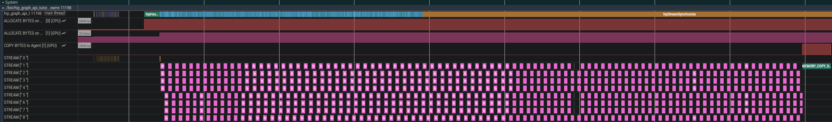
While projections process in parallel, there are visible gaps between operations. These gaps represent overhead caused by scheduling and launching the operations. In the next section, you will eliminate these gaps by capturing streams into a graph.

Step 3: Converting to graphs via stream capture

Stream capture is a feature that allows you to record a sequence of GPU operations (kernel launches, memory copies, etc.) into a HIP Graph, which can later be executed as a single, optimized unit. Open the file src/main_graph_capture.hip, which contains the code from the previous subsection, with a few changes that allow you to capture the streams into a single graph.

Before the main loop, declare graph-specific variables:

auto graphCreated = false;
auto graphExec = hipGraphExec_t{};
auto graphFinalCreated = false;
auto graphExecFinal = hipGraphExec_t{};
auto graphStream = hipStream_t{};
hip_check(hipStreamCreate(&graphStream));

graphExec and graphExecFinal will be instances of the graph template that you will create in the following steps. You will typically instantiate a graph template once and update its parameters for repeated launches. If the graph topology changes, you will need a new instance. The graphStream will launch the final graph instances.

Inside the main loop, activate capture mode on the first stream:

// Capture the current batch into a graph template
auto graph = hipGraph_t{};
hip_check(hipStreamBeginCapture(streams.at(0), hipStreamCaptureModeGlobal));

To capture multiple streams, use events to implement the fork-join pattern:

// Fork: Record events on stream 0, then have other streams wait
for(auto streamIdx = 1; streamIdx < batchSize; ++streamIdx)
{
    auto forkEvent = hipEvent_t{};
    hip_check(hipEventCreate(&forkEvent));
    hip_check(hipEventRecord(forkEvent, streams.at(0)));
    hip_check(hipStreamWaitEvent(streams.at(streamIdx), forkEvent));
    hip_check(hipEventDestroy(forkEvent)); // Can destroy after wait is recorded
}

This creates dependencies between streams, activating capture mode on the additional streams and ensuring they are all part of the same graph.

The processing pipeline itself remains unchanged.

After recording all operations of the current batch, join the streams:

// Join: Record events on all streams except stream 0, then have stream 0 wait
for(auto streamIdx = 1; streamIdx < batchSize; ++streamIdx)
{
    auto joinEvent = hipEvent_t{};
    hip_check(hipEventCreate(&joinEvent));
    hip_check(hipEventRecord(joinEvent, streams.at(streamIdx)));
    hip_check(hipStreamWaitEvent(streams.at(0), joinEvent));
    hip_check(hipEventDestroy(joinEvent)); // Can destroy after wait is recorded
}

Then stop capturing:

// Stop capturing -- this will stop capturing on all streams
hip_check(hipStreamEndCapture(streams.at(0), &graph));

The graph template is now complete. In order to execute the recorded operations, you need to instantiate the graph and execute it on the graphStream. The graph template can be safely destroyed after instantiating:

if(!graphCreated)
{
    hip_check(hipGraphDebugDotPrint(graph, "graph_capture.dot", hipGraphDebugDotFlagsVerbose));

    hip_check(hipGraphInstantiate(&graphExec, graph, nullptr, nullptr, 0));
    hip_check(hipGraphDestroy(graph));
    hip_check(hipGraphLaunch(graphExec, graphStream));
    graphCreated = true;
}

Tip

Use hipGraphDebugDotPrint() to save a graph’s topology into a *.dot file. The resulting file contains a DOT description which can be processed with Graphviz or visualized with several tools. For example:

dot -Tpng graph_capture.dot -o graph_capture.png

Instantiating a graph is a relatively costly operation. However, you need to update the parameters whenever a new batch is processed. Since the graph templates are the same for all batches (i.e., the topology of the resulting graph does not change), it is sufficient to update the existing graph instance’s parameters instead of creating a new instance:

else
{
    // Update existing executable graph after each iteration with new input data
    auto result = hipGraphExecUpdateResult{};
    auto errorNode = hipGraphNode_t{};
    hip_check(hipGraphExecUpdate(graphExec, graph, &errorNode, &result));
    if(result != hipGraphExecUpdateSuccess)
    {
        auto msg = std::string{"Failed to update graph: "};
        switch(result)
        {
        case hipGraphExecUpdateError:
            msg += "Invalid value.";
            break;
        case hipGraphExecUpdateErrorFunctionChanged:
            msg += "Function of kernel node changed.";
            break;
        case hipGraphExecUpdateErrorNodeTypeChanged:
            msg += "Type of node changed.";
            break;
        case hipGraphExecUpdateErrorNotSupported:
            msg += "Something about the node is not supported.";
            break;
        case hipGraphExecUpdateErrorParametersChanged:
            msg += "Unsupported parameter change.";
            break;
        case hipGraphExecUpdateErrorTopologyChanged:
            msg += "Graph topology changed.";
            break;
        case hipGraphExecUpdateErrorUnsupportedFunctionChange:
            msg += "Unsupported change of kernel node function.";
            break;
        default:
            msg += "Unknown error.";
            break;
        }
        throw std::runtime_error{msg};
    }
    hip_check(hipGraphDestroy(graph));
    hip_check(hipGraphLaunch(graphExec, graphStream));
}

Should the graph’s topology change between iterations, it is necessary to create a new graph instance. In your application’s case, this can happen when the number of projections is not evenly divisible by the number of asynchronous engines:

hip_check(hipGraphDebugDotPrint(graph, "graph_capture_final.dot", hipGraphDebugDotFlagsVerbose));

// Incomplete batch: topology changed, must instantiate new executable graph
hip_check(hipGraphInstantiate(&graphExecFinal, graph, nullptr, nullptr, 0));
hip_check(hipGraphDestroy(graph));
hip_check(hipGraphLaunch(graphExecFinal, graphStream));

Creating a trace

Now you have successfully converted the processing pipeline into an executable graph. You can examine the effects of this change and generate another trace:

rocprofv3 -o graph_capture -d outDir -f pftrace --hip-trace --kernel-trace --memory-copy-trace --memory-allocation-trace -- ./HIP-Doc/Tutorials/graph_api/src/hip_graph_api_tutorial_graph_capture

Analyzing the trace

Opening the resulting trace file outDir/graph_capture_results.pftrace with Perfetto shows a significant change:

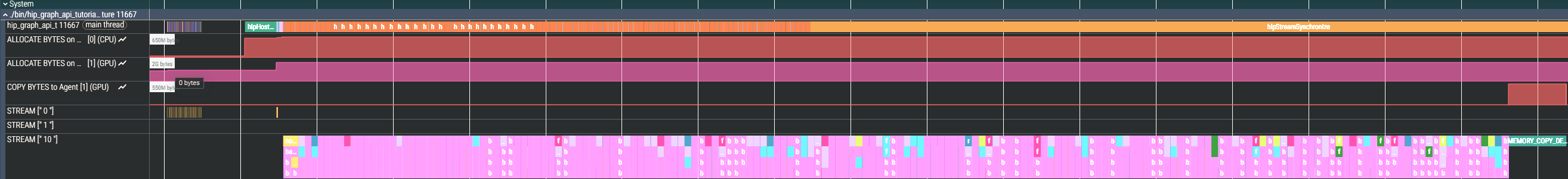
The gaps have disappeared! By capturing all operations of a batch into a single graph, you have successfully eliminated the launching and scheduling overhead previously observed in the stream-based variant.

A limitation of stream capture is that it preserves stream ordering even when unnecessary. Operations that could run in parallel still execute sequentially. Another approach to graphs is manual construction. This is quite verbose but also offers much more control over dependencies and parallelism.

Step 4: Manual graph creation (advanced)

Open src/main_graph_creation.hip and find the main loop. The code here differs from the other variants: rather than capturing streams into graphs, you will build the graph manually. Consider how the weighting kernel is invoked through a kernel node:

void* weightingKernelParams[] =
{
    static_cast<void*>(&proj),
    static_cast<void*>(&projPitch),
    static_cast<void*>(&projGeom.dim),
    static_cast<void*>(&projGeom.d_sd),
    static_cast<void*>(&projGeom.d_so),
    static_cast<void*>(&projGeom.minCoord),
    static_cast<void*>(&projGeom.pixelDim)
};
auto weightingKernelNodeParams = hipKernelNodeParams{};
weightingKernelNodeParams.blockDim = threadsPerBlock;
weightingKernelNodeParams.extra = nullptr;
weightingKernelNodeParams.func = reinterpret_cast<void*>(weighting_kernel);
weightingKernelNodeParams.gridDim = blocksPerGrid;
weightingKernelNodeParams.kernelParams = weightingKernelParams;
weightingKernelNodeParams.sharedMemBytes = 0;
auto weightingKernelNode = hipGraphNode_t{};
hip_check(hipGraphAddKernelNode(
    &weightingKernelNode, graph, &logTransformationKernelNode, 1, &weightingKernelNodeParams
));

You create an array of void* pointers containing the kernel parameters. Next, configure the kernel launch parameters: grid and block dimensions, the kernel function pointer, and the dynamic shared memory size. Finally, add the kernel node to the graph template. Note the &logTransformationKernelNode, 1 part: this is how you specify a dependency from the preceding log transformation kernel node to the weighting kernel node.

Note

For specifying multiple dependencies, you would pass an array of hipGraphNode_t objects and the number of nodes inside the array to hipGraphAddKernelNode().

The HIP graph API supports multiple different node types. For example, this is how a memset node is set up:

auto expandedMemsetNodeParams = hipMemsetParams{};
expandedMemsetNodeParams.dst = static_cast<void*>(expanded);
expandedMemsetNodeParams.elementSize = sizeof(float);
expandedMemsetNodeParams.height = projGeom.dimFFT.y;
expandedMemsetNodeParams.pitch = expandedPitch;
expandedMemsetNodeParams.value = 0;
expandedMemsetNodeParams.width = projGeom.dimFFT.x;
auto expandedMemsetNode = hipGraphNode_t{};
hip_check(hipGraphAddMemsetNode(
    &expandedMemsetNode, graph, &weightingKernelNode, 1, &expandedMemsetNodeParams
));

Note

Despite the different construction method, graph instantiation and updates work exactly as before. You can find the same patterns at the loop’s end.

Adding hipFFT nodes

While hipFFT provides graph-safe functionality, it does not support manual node creation. Integrating hipFFT into the graph requires a workaround using stream capture with additional bookkeeping.

You capture the graph state before and after hipFFT operations, then identify the nodes hipFFT added:

Step 1: Save existing nodes

Record all current graph nodes in a sorted std::set:

// Before capturing the FFT operations, obtain the set of nodes already present in the graph
auto nodesBeforeForward = std::vector<hipGraphNode_t>{};
auto numNodesBeforeForward = std::size_t{};
hip_check(hipGraphGetNodes(graph, nullptr, &numNodesBeforeForward));
nodesBeforeForward.resize(numNodesBeforeForward);
hip_check(hipGraphGetNodes(graph, nodesBeforeForward.data(), &numNodesBeforeForward));
auto nodesBeforeForwardSorted = std::set<hipGraphNode_t>{
    std::begin(nodesBeforeForward), std::end(nodesBeforeForward)
};

Step 2: Capture hipFFT operations

hip_check(hipStreamBeginCaptureToGraph(
    stream, graph, &transformedMemsetNode, nullptr, 1, hipStreamCaptureModeGlobal));

auto& forward = forwardPlans.at(branchIdx);
hipfft_check(hipfftExecR2C(forward, expanded, transformed));

hip_check(hipStreamEndCapture(stream, &graph));

Step 3: Get updated node list

// Obtain nodes in graph again, the new nodes will be our dependencies for the next step
auto nodesAfterForward = std::vector<hipGraphNode_t>{};
auto numNodesAfterForward = std::size_t{};
hip_check(hipGraphGetNodes(graph, nullptr, &numNodesAfterForward));
nodesAfterForward.resize(numNodesAfterForward);
hip_check(hipGraphGetNodes(graph, nodesAfterForward.data(), &numNodesAfterForward));
auto nodesAfterForwardSorted = std::set<hipGraphNode_t>{
    std::begin(nodesAfterForward), std::end(nodesAfterForward)
};

Step 4: Find new nodes

Compute the difference between both node sets:

// Compute difference between both sets
auto forwardFFTNodes = std::vector<hipGraphNode_t>{};
std::set_difference(std::begin(nodesAfterForwardSorted), std::end(nodesAfterForwardSorted),
                    std::begin(nodesBeforeForwardSorted), std::end(nodesBeforeForwardSorted),
                    std::back_inserter(forwardFFTNodes));

Step 5: Identify the leaf node

Find hipFFT’s final node for dependency tracking:

// Find leaf node in difference set
auto forwardLeafNode = *(std::find_if(std::begin(forwardFFTNodes), std::end(forwardFFTNodes), is_leaf));

The leaf detection logic checks if a node has no outgoing edges:

auto is_leaf = [](hipGraphNode_t node)
{
    auto numDependentNodes = std::size_t{};
    hip_check(hipGraphNodeGetDependentNodes(node, nullptr, &numDependentNodes));
    return numDependentNodes == 0;
};

With hipFFT integrated and its leaf node identified, subsequent nodes can establish proper dependencies.

Note

You can also capture hipFFT operations into a separate graph template, then add it to the main graph as a child graph using hipGraphAddChildGraphNode(). The approach above adds hipFFT nodes directly to the main graph as first-class nodes. A child graph acts as a single node that expands recursively into its components. The scheduler may handle these approaches differently, potentially affecting performance.

Creating a trace

Now you have manually implemented the processing pipeline with the graph API. You can examine the result by generating another trace:

rocprofv3 -o graph_creation -d outDir -f pftrace --hip-trace --kernel-trace --memory-copy-trace --memory-allocation-trace -- ./HIP-Doc/Tutorials/graph_api/src/hip_graph_api_tutorial_graph_creation

Analyzing the trace

Opening the resulting trace file outDir/graph_creation_results.pftrace with Perfetto shows a similar trace to what you achieved with the capture variant:

Like before, the kernels are executed en bloc. By creating nodes for all operations in the processing pipeline, you avoided the launching and scheduling overhead you previously observed in the stream-based variant.

Updating individual nodes

The code presented in this tutorial updates the entire graph instance for each new batch. Applications that require updates to only a small subset of nodes might experience excessive overhead. For these cases, the HIP Graph API provides the following methods for updating individual nodes:

• hipGraphExecChildGraphNodeSetParams()

• hipGraphExecEventRecordNodeSetEvent()

• hipGraphExecEventWaitNodeSetEvent()

• hipGraphExecExternalSemaphoresSignalNodeSetParams()

• hipGraphExecExternalSemaphoresWaitNodeSetParams()

• hipGraphExecHostNodeSetParams()

• hipGraphExecKernelNodeSetParams()

• hipGraphExecMemcpyNodeSetParams()

• hipGraphExecMemcpyNodeSetParams1D()

• hipGraphExecMemcpyNodeSetParamsFromSymbol()

• hipGraphExecMemcpyNodeSetParamsToSymbol()

• hipGraphExecMemsetNodeSetParams()

• hipGraphExecNodeSetParams()

Conclusion

When an application has predictable, repetitive workflows, transitioning from streams to graphs can significantly reduce launch overhead and improve performance. HIP provides two approaches for creating graphs: stream capture and explicit graph construction.

Stream capture converts existing stream-based code into a graph by recording the operations between start and stop capture calls. This approach minimizes code changes and works well when your application already has a graph-like structure with clear dependencies.

Explicit graph construction involves manually creating nodes and defining edges between them using the graph API. While this approach requires more code changes and is more verbose, it provides fine-grained control over dependencies and allows for optimizations that might not be possible with stream capture. This method is ideal when you need precise control over the graph topology or when working with complex dependency patterns.

Tip

Choose stream capture for quick conversions of existing code with minimal changes. Choose explicit construction when you need maximum control and optimization opportunities.

Resources

• HIP Programming Guide’s section on HIP graphs

• HIP graph API reference

References

[FeDK84]

12. 1. Feldkamp, L. C. Davis and J. W. Kress: “Practical cone-beam algorithm”. In Journal of the Optical Society of America A, vol. 1, no. 6, pp. 612-619, June 1984, DOI 10.1364/JOSAA.1.000612.

[ShLo74]

12. 1. Shepp and B. F. Logan: “The Fourier reconstruction of a head section”. In IEEE Transactions on Nuclear Science, vol. 21, no. 3, pp. 21-43, June 1974, DOI 10.1109/TNS.1974.6499235.