AMD Instinct MI300X workload optimization

Applies to Linux

2024-08-06

61 min read time

This document provides guidelines for optimizing the performance of AMD Instinct™ MI300X accelerators, with a particular focus on GPU kernel programming, high-performance computing (HPC), and deep learning operations using PyTorch. It delves into specific workloads such as model inference, offering strategies to enhance efficiency.

The following topics highlight auto-tunable configurations that streamline optimization as well as advanced techniques like Triton kernel optimization for meticulous tuning.

Workload tuning strategy

By following a structured approach, you can systematically address performance issues and enhance the efficiency of your workloads on AMD Instinct MI300X accelerators.

Measure the current workload

Begin by evaluating the performance of your workload in its current state. This involves running benchmarks and collecting performance data to establish a baseline. Understanding how your workload behaves under different conditions provides critical insights into where improvements are needed.

Identify tuning requirements

Analyze the collected performance data to identify areas where tuning is required. This could involve detecting bottlenecks in CPU, GPU, memory, or data transfer. Understanding these requirements will help direct your optimization efforts more effectively.

Profiling is a fundamental step in workload tuning. It allows you to gather detailed information about how your workload utilizes system resources, and where potential inefficiencies lie. Profiling tools can provide insights into both high-level and granular performance metrics. See Profiling tools.

High-level profiling tools

For a broad overview, use tools like the PyTorch Profiler, which helps in understanding how PyTorch operations are executed and where time is spent. This is particularly useful for developers new to workload tuning, as it provides a comprehensive view without requiring in-depth knowledge of lower-level operations.

Kernel-level profiling tools

When profiling indicates that GPUs are a performance bottleneck, delve deeper into kernel-level profiling. Tools such as the ROCr Debug Agent, ROCProfiler, and Omniperf offer detailed insights into GPU kernel execution. These tools can help isolate problematic GPU operations and provide data needed for targeted optimizations.

Analyze and tune

Based on the insights gained from profiling, focus your tuning efforts on the identified bottlenecks. This might involve optimizing specific kernel operations, adjusting memory access patterns, or modifying computational algorithms.

The following subsections discuss optimization ranging from high-level and more automated strategies to more involved, hands-on optimization.

Optimize model inference with vLLM

vLLM provides tools and techniques specifically designed for efficient model inference on AMD Instinct MI300X accelerators. See vLLM inference for installation guidance. Optimizing performance with vLLM involves configuring tensor parallelism, leveraging advanced features, and ensuring efficient execution. Here’s how to optimize vLLM performance:

• Tensor parallelism: Configure the tensor-parallel-size parameter to distribute tensor computations across multiple GPUs. Adjust parameters such as batch-size, input-len, and output-len based on your workload.

• Configuration for vLLM: Set parameters according to workload requirements. Benchmark performance to understand characteristics and identify bottlenecks.

• Benchmarking and performance metrics: Measure latency and throughput to evaluate performance.

Auto-tunable configurations

Auto-tunable configurations can significantly streamline performance optimization by automatically adjusting parameters based on workload characteristics. For example:

• PyTorch: Utilize PyTorch’s built-in auto-tuning features, such as the TunableOp module, which helps in optimizing operation performance by exploring different configurations.

• MIOpen: Leverage MIOpen’s auto-tuning capabilities for convolutional operations and other primitives to find optimal settings for your specific hardware.

• Triton: Use Triton’s auto-tuning features to explore various kernel configurations and automatically select the best-performing ones.

Manual tuning

Advanced developers can manually adjust parameters and configurations to optimize performance. Both Triton and HIP involve manual tuning aspects.

• ROCm libraries: Optimize GPU performance by adjusting various parameters and configurations within ROCm libraries. This approach involves hands-on optimization to maximize efficiency for specific workloads.

• Triton: Tune Triton kernels by adjusting parameters tailored to your workload to optimize GPU resource utilization and better leverage specific hardware features.

• HIP: Profile and optimize HIP kernels by optimizing parallel execution, memory access patterns, and other aspects.

Iterate and validate

Optimization is an iterative process. After applying tuning changes, re-profile the workload to validate improvements and ensure that the changes have had the desired effect. Continuous iteration helps refine the performance gains and address any new bottlenecks that may emerge.

Profiling tools

AMD profiling tools provide valuable insights into how efficiently your application utilizes hardware and help diagnose potential bottlenecks that contribute to poor performance. Developers targeting AMD GPUs have multiple tools available depending on their specific profiling needs.

• ROCProfiler tool collects kernel execution performance metrics. For more information, see the ROCProfiler documentation.

• Omniperf builds upon ROCProfiler but provides more guided analysis. For more information, see Omniperf documentation.

Refer to Profiling and debugging to explore commonly used profiling tools and their usage patterns.

Once performance bottlenecks are identified, you can implement an informed workload tuning strategy. If kernels are the bottleneck, consider:

• Auto-tuning in PyTorch with TunableOp

• Auto-tuning in MIOpen

• Triton auto-tunable kernel configurations

If auto-tuning does not meet your requirements, consider Triton kernel performance optimization.

If the issue is multi-GPU scale-out, try RCCL tuning and configuration.

This section discusses profiling and debugging tools and some of their common usage patterns with ROCm applications.

PyTorch Profiler

PyTorch Profiler can be invoked inside Python scripts, letting you collect CPU and GPU performance metrics while the script is running. See the PyTorch Profiler tutorial for more information.

You can then visualize and view these metrics using an open-source profile visualization tool like Perfetto UI.

1. Use the following snippet to invoke PyTorch Profiler in your code.

   import torch
   import torchvision.models as models
   from torch.profiler import profile, record_function, ProfilerActivity
   model = models.resnet18().cuda()
   inputs = torch.randn(2000, 3, 224, 224).cuda()
   
   with profile(activities=[ProfilerActivity.CPU, ProfilerActivity.CUDA]) as prof:
       with record_function("model_inference"):
           model(inputs)
   prof.export_chrome_trace("resnet18_profile.json")
   

2. Profile results in resnet18_profile.json can be viewed by the Perfetto visualization tool. Go to https://ui.perfetto.dev and import the file. In your Perfetto visualization, you’ll see that the upper section shows transactions denoting the CPU activities that launch GPU kernels while the lower section shows the actual GPU activities where it processes the resnet18 inferences layer by layer.

   

   Perfetto trace visualization example.

ROCm profiling tools

Heterogenous systems, where programs run on both CPUs and GPUs, introduce additional complexities. Understanding the critical path and kernel execution is all the more important; so, performance tuning is a necessary component in the benchmarking process.

With AMD’s profiling tools, developers are able to gain important insight into how efficiently their application is using hardware resources and effectively diagnose potential bottlenecks contributing to poor performance. Developers working with AMD Instinct accelerators have multiple tools depending on their specific profiling needs; these are:

• ROCProfiler

• Omniperf

• Omnitrace

ROCProfiler

ROCProfiler is primarily a low-level API for accessing and extracting GPU hardware performance metrics, commonly called performance counters. These counters quantify the performance of the underlying architecture showcasing which pieces of the computational pipeline and memory hierarchy are being utilized.

Your ROCm installation contains a script or executable command called rocprof which provides the ability to list all available hardware counters for your specific accelerator or GPU, and run applications while collecting counters during their execution.

This rocprof utility also depends on the ROCTracer and ROC-TX libraries, giving it the ability to collect timeline traces of the accelerator software stack as well as user-annotated code regions.

Note

rocprof is a CLI-only utility so input and output takes the format of .txt and CSV files. These formats provide a raw view of the data and puts the onus on the user to parse and analyze. Therefore, rocprof gives the user full access and control of raw performance profiling data, but requires extra effort to analyze the collected data.

Omniperf

Omniperf is a system performance profiler for high-performance computing (HPC) and machine learning (ML) workloads using Instinct accelerators. Under the hood, Omniperf uses ROCProfiler to collect hardware performance counters. The Omniperf tool performs system profiling based on all approved hardware counters for Instinct accelerator architectures. It provides high level performance analysis features including System Speed-of-Light, IP block Speed-of-Light, Memory Chart Analysis, Roofline Analysis, Baseline Comparisons, and more.

Omniperf takes the guesswork out of profiling by removing the need to provide text input files with lists of counters to collect and analyze raw CSV output files as is the case with ROC-profiler. Instead, Omniperf automates the collection of all available hardware counters in one command and provides a graphical interface to help users understand and analyze bottlenecks and stressors for their computational workloads on AMD Instinct accelerators.

Note

Omniperf collects hardware counters in multiple passes, and will therefore re-run the application during each pass to collect different sets of metrics.

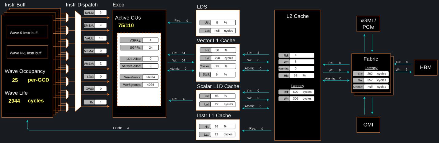
Omniperf memory chat analysis panel.

In brief, Omniperf provides details about hardware activity for a particular GPU kernel. It also supports both a web-based GUI or command-line analyzer, depending on your preference.

Omnitrace

Omnitrace is a comprehensive profiling and tracing tool for parallel applications, including HPC and ML packages, written in C, C++, Fortran, HIP, OpenCL, and Python which execute on the CPU or CPU and GPU. It is capable of gathering the performance information of functions through any combination of binary instrumentation, call-stack sampling, user-defined regions, and Python interpreter hooks.

Omnitrace supports interactive visualization of comprehensive traces in the web browser in addition to high-level summary profiles with mean/min/max/stddev statistics. Beyond runtime information, Omnitrace supports the collection of system-level metrics such as CPU frequency, GPU temperature, and GPU utilization. Process and thread level metrics such as memory usage, page faults, context switches, and numerous other hardware counters are also included.

Tip

When analyzing the performance of an application, it is best not to assume you know where the performance bottlenecks are and why they are happening. Omnitrace is the ideal tool for characterizing where optimization would have the greatest impact on the end-to-end execution of the application and to discover what else is happening on the system during a performance bottleneck.

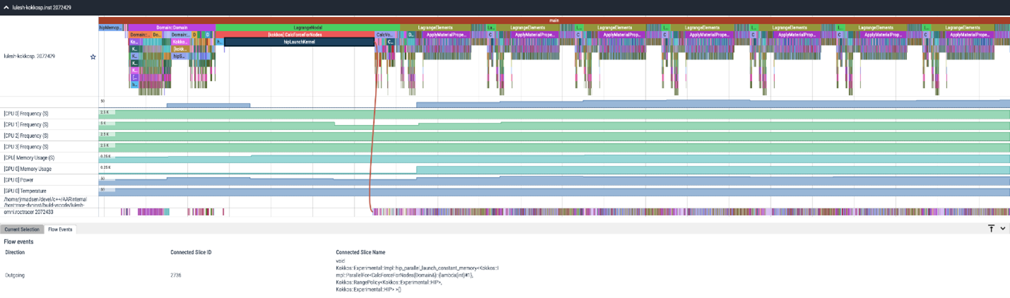
Omnitrace timeline trace example.

For details usage and examples of using these tools, refer to the Introduction to profiling tools for AMD hardware developer blog.

vLLM performance optimization

The following performance tips are not specific to vLLM – they are general but relevant in this context. You can tune the following vLLM parameters to achieve optimal request latency and throughput performance.

• As described in Environment variables, the environment variable HIP_FORCE_DEV_KERNARG can improve vLLM performance. Set it to export HIP_FORCE_DEV_KERNARG=1.

• vLLM is based on PyTorch. Therefore, the suggestions in the TunableOp section are also applicable to vLLM tuning as long as the PyTorch version is 2.3 or later.

• Set the RCCL environment variable NCCL_MIN_NCHANNELS to 112 to increase the number of channels on MI300X to potentially improve the performance.

The following subsections describe vLLM-specific suggestions for performance.

• tensor_parallel_size

• max_model_len

• gpu_memory_utilization

• enforce_eager

• kv_cache_dtype

• input_len

• output_len

• enforce_eager

• batch_size

• enable_chunked_prefill

Refer to vLLM documentation for additional performance tips. vLLM inference describes vLLM usage with ROCm.

Maximize throughput

The general guideline is to maximize per-node throughput. Specify proper GPU memory utilization to run as many instances of vLLM as possible on a single GPU. However, too many instances can result in no memory for KV-cache.

You can run vLLM on MI300X (gfx942), for example, using model weights for llama2 (7b, 13b, 70b) and llama3 models (8b, 70b).

As described in the AMD Instinct MI300X Accelerator data sheet, the GPU memory capacity is 192 GB. This means you can run llama2-70b and llama3-70b models on one GPU.

To maximize the accumulated throughput, you can also run eight instances vLLM simultaneously on one MI300X node (with eight GPUs). To do so, use the GPU isolation environment variable CUDA_VISIBLE_DEVICES.

For example, this script runs eight instances of vLLM for throughput benchmarking at the same time:

for i in $(seq 0 7);
do
    CUDA_VISIBLE_DEVICES="$i" python3 /app/vllm/benchmarks/benchmark_throughput.py -tp 1 --dataset "/path/to/dataset/ShareGPT_V3_unfiltered_cleaned_split.json" --model /path/to/model &
done

Run two instances of llama3-8b model at the same time on one single GPU by specifying --gpu-memory-utilization to 0.4 (40%), as below (on GPU 0):

CUDA_VISIBLE_DEVICES=0 python3
/vllm-workspace/benchmarks/benchmark_throughput.py --gpu-memory-utilization
0.4 --dataset
"/path/to/dataset/ShareGPT_V3_unfiltered_cleaned_split.json" --model
/path/to/model &

CUDA_VISIBLE_DEVICES=0 python3
/vllm-workspace/benchmarks/benchmark_throughput.py --gpu-memory-utilization
0.4 --dataset
"/path/to/dataset/ShareGPT_V3_unfiltered_cleaned_split.json" --model
/path/to/model &

Similarly, use the CUDA_VISIBLE_DEVICES environment variable to specify which GPU (0-7) will run those instances.

Run vLLM on multiple GPUs

The two main reasons to use multiple GPUs:

• The model size is too big to run vLLM using one GPU as it results CUDA/HIP Out of Memory.

• To achieve better latency.

To run one vLLM instance on multiple GPUs, use the -tp or --tensor-parallel-size option to specify multiple GPUs. Optionally, use the CUDA_VISIBLE_DEVICES environment variable to specify the GPUs.

For example, you can use two GPUs to start an API server on port 8000 as below:

python -m vllm.entrypoints.api_server --model /path/to/model --dtype
float16 -tp 2 --port 8000 &

To achieve both latency and throughput performance for serving, you can run multiple API servers on different GPUs by specifying different ports for each server and use CUDA_VISIBLE_DEVICES to specify the GPUs for each server, for example:

CUDA_VISIBLE_DEVICES=0,1 python -m vllm.entrypoints.api_server --model
/path/to/model --dtype float16 -tp 2 --port 8000 &

CUDA_VISIBLE_DEVICES=2,3 python -m vllm.entrypoints.api_server --model
/path/to/model --dtype float16 -tp 2 --port 8001 &

See Optimize tensor parallelism and GEMM performance for additional optimization suggestions.

Choose different attention backends

vLLM on ROCm supports three different attention backends, each suitable for different use cases and performance requirements:

• Triton Flash Attention - For benchmarking, run vLLM scripts at least once as a warm-up step so Triton can perform auto-tuning before collecting benchmarking numbers. This is the default setting.

• Composable Kernel (CK) Flash Attention - To use CK Flash Attention, specify the environment variable as export VLLM_USE_TRITON_FLASH_ATTN=0.

• PyTorch naive attention - To use naive attention (PyTorch SDPA math backend), either build the Docker image without Flash Attention by passing --build-arg BUILD_FA="0" during Docker build, or pip uninstall flash-attn inside the container, and export VLLM_USE_TRITON_FLASH_ATTN=0 when running the vLLM instance.

Refer to Model acceleration libraries to learn more about Flash Attention with Triton or CK backends.

Use fp8 KV-cache data type

Using fp8 kv-cache dtype can improve performance as it reduces the size of kv-cache. As a result, it reduces the cost required for reading and writing the kv-cache.

To use this feature, specify --kv-cache-dtype as fp8.

To specify the quantization scaling config, use the --quantization-param-path parameter. If the parameter isn’t specified, the default scaling factor of 1 is used, which can lead to less accurate results. To generate kv-cache scaling JSON file, see FP8 KV Cache in the vLLM GitHub repository.

Two sample Llama scaling configuration files are in vLLM for llama2-70b and llama2-7b.

If building the vLLM using Dockerfile.rocm for llama2-70b scale config, find the file at /vllm-workspace/tests/fp8_kv/llama2-70b-fp8-kv/kv_cache_scales.json at runtime.

Below is a sample command to run benchmarking with this feature enabled for the llama2-70b model:

python3 /vllm-workspace/benchmarks/benchmark_throughput.py --model
/path/to/llama2-70b-model --kv-cache-dtype "fp8"
--quantization-param-path
"/vllm-workspace/tests/fp8_kv/llama2-70b-fp8-kv/kv_cache_scales.json"
--input-len 512 --output-len 256 --num-prompts 500

Note

As of the writing of this document, this feature enhances performance when a single GPU is used (with a tensor-parallel size of 1).

Enable chunked prefill

Another vLLM performance tip is to enable chunked prefill to improve throughput. Chunked prefill allows large prefills to be chunked into smaller chunks and batched together with decode requests.

You can enable the feature by specifying --enable-chunked-prefill in the command line or setting enable_chunked_prefill=True in the LLM constructor.

As stated in vLLM’s documentation,, you can tune the performance by changing max_num_batched_tokens. By default, it is set to 512 and optimized for ITL (inter-token latency). Smaller max_num_batched_tokens achieves better ITL because there are fewer prefills interrupting decodes. Higher max_num_batched_tokens achieves better TTFT (time to the first token) as you can put more prefill to the batch.

You might experience noticeable throughput improvements when benchmarking on a single GPU or 8 GPUs using the vLLM throughput benchmarking script along with the ShareGPT dataset as input.

In the case of fixed input-len/output-len, for some configurations, enabling chunked prefill increases the throughput. For some other configurations, the throughput may be worse and elicit a need to tune parameter max_num_batched_tokens (for example, increasing max_num_batched_tokens value to 4096 or larger).

Optimize tensor parallelism and GEMM performance

You can use tensor parallelism to improve performance in model inference tasks by distributing tensor computations across multiple GPUs. The ROCm vLLM fork supports two modes to run tensor parallelism: ray and torchrun which (the default in ROCm for performance reasons).

• To use torchrun, use the following command where $WORLD_SIZE is the number of GPUs or number of workers to use per node. In the case of nnodes=1 (that is, the number of nodes is 1), it’s the same as the tensor-parallel-size or -tp.

  torchrun --standalone --nnodes=1 --nproc-per-node=$WORLD_SIZE YOUR_PYTHON_SCRIPT.py (--tensor-parallel-size $WORLD_SIZE .. other_script_args...)
  

• To use ray, specify the --worker-use-ray flag. The following script example uses torchrun to run latency benchmarking using ray for input-len of 512, output-len of 512, and batch-size of 1:

  tp=$1
  
  torchrun --standalone --nnodes=1 --nproc-per-node=$tp benchmarks/benchmark_latency.py --worker-use-ray --model $MODEL --batch-size 1 --input-len 512 --output-len 512 --tensor-parallel-size $tp --num-iters 10
  

  The first parameter of the script tp specifies the tensor-parallel size (1 to 8).

GEMM tuning steps

This section describes the process of optimizing the parameters and configurations of GEMM operations to improve their performance on specific hardware. This involves finding the optimal settings for memory usage, computation, and hardware resources to achieve faster and more efficient matrix multiplication.

Follow these steps to perform GEMM tuning with ROCm vLLM:

1. Set various environment variables to specify paths for tuning files and enable debugging options:

   export VLLM_UNTUNE_FILE="/tmp/vllm_untuned.csv"
   
   export VLLM_TUNE_FILE="$(pwd)/vllm/tuned.csv"
   
   export HIP_FORCE_DEV_KERNARG=1
   
   export DEBUG_CLR_GRAPH_PACKET_CAPTURE=1
   

2. Perform a tuning run:

   VLLM_TUNE_GEMM=1 torchrun --standalone --nnodes=1 --nproc-per-node=8 vllm/benchmarks/benchmark_latency.py --batch-size 1 --input-len 2048 --output-len 128 --model /models/llama-2-70b-chat-hf/ -tp 8
   
   python $PATH_TO_GRADLIB/gemm_tuner.py --input /tmp/vllm_untuned.csv --tuned_file vllm/tuned.csv
   

   $PATH_TO_GRADLIB is the installation path of gradlib. To find where gradlib is, you can run pip show gradlib and then update the above path to something like /opt/conda/envs/py_3.9/lib/python3.9/site-packages/gradlib/gemm_tuner.py

3. Do a measurement run to verify performance improvements:

   VLLM_TUNE_GEMM=0 torchrun --standalone --nnodes=1 --nproc-per-node=8 vllm/benchmarks/benchmark_latency.py --batch-size 1 --input-len 2048 --output-len 128 --model /models/llama-2-70b-chat-hf/ -tp 8
   

PyTorch TunableOp

TunableOp is a feature used to define and optimize kernels that can have tunable parameters. This is useful in optimizing the performance of custom kernels by exploring different parameter configurations to find the most efficient setup. See more about PyTorch TunableOp in Model acceleration libraries.

You can easily manipulate the behavior TunableOp through environment variables, though you could use the C++ interface at::cuda::tunable::getTuningContext(). A Python interface to the TuningContext does not yet exist.

The three most important environment variables are:

PYTORCH_TUNABLEOP_ENABLED

Default is 0. Set to 1 to enable. This is the main on/off switch for all TunableOp implementations.

PYTORCH_TUNABLEOP_TUNING

Default is 1. Set to 0 to disable. When enabled, if a tuned entry isn’t found, run the tuning step and record the entry.

PYTORCH_TUNABLEOP_VERBOSE

Default is 0. Set to 1 if you want to see TunableOp in action.

Use these environment variables to enable TunableOp for any applications or libraries that use PyTorch (2.3 or later). For more information, see pytorch/pytorch on GitHub.

You can check how TunableOp performs in two steps:

1. Enable TunableOp and tuning. Optionally enable verbose mode:

   PYTORCH_TUNABLEOP_ENABLED=1 PYTORCH_TUNABLEOP_VERBOSE=1 your_script.sh
   

2. Enable TunableOp and disable tuning and measure.

   PYTORCH_TUNABLEOP_ENABLED=1  PYTORCH_TUNABLEOP_TUNING=0 your_script.sh
   

PyTorch inductor Triton tuning knobs

The following are suggestions for optimizing matrix multiplication (GEMM) and convolution (conv) operations in PyTorch using inductor, a part of the PyTorch compilation framework. The goal is to leverage Triton to achieve better performance.

Learn more about TorchInductor environment variables and usage in PyTorch documentation.

To tune Triton kernels with gemm and convolution ops (conv), use the torch.compile function with the max-autotune mode. This benchmarks a predefined list of Triton configurations and selects the fastest one for each shape. See the configurations in PyTorch source code:

• conv configs for max-autotune

• matmul configs for max-autotune

Note

Triton is not used if regular MIOpen or rocBLAS performs faster for a specific operation.

• Set torch._inductor.config.max_autotune = True or TORCHINDUCTOR_MAX_AUTOTUNE=1.

• Or, for more fine-grained control:

  torch._inductor.config.max_autotune_gemm = True

  To enable tuning or lowering of mm/convs.

  torch._inductor.config.max_autotune.pointwise = True

  To enable tuning for pointwise/reduction ops.

  torch._inductor.max_autotune_gemm_backends or TORCHINDUCTOR_MAX_AUTOTUNE_GEMM_BACKENDS

  Selects the candidate backends for mm auto-tuning. Defaults to TRITON,ATEN. Limiting this to TRITON might improve performance by enabling more fused mm kernels instead of going to rocBLAS.

• For further mm tuning, tuning coordinate_descent might improve performance.

  torch._inductor.config.coordinate_descent_tuning = True or TORCHINDUCTOR_COORDINATE_DESCENT_TUNING=1

• Inference can see large improvements on AMD GPUs by utilizing torch._inductor.config.freezing=True or the TORCHINDUCTOR_FREEZING=1 variable, which in-lines weights as constants and enables constant folding optimizations.

• Enabling inductor’s cpp_wrapper might improve overhead. This generates C++ code which launches Triton binaries directly with hipModuleLaunchKernel and relies on hipification.

  torch._inductor.config.cpp_wrapper=True or TORCHINDUCTOR_CPP_WRAPPER=1

• Convolution workloads may see a performance benefit by specifying torch._inductor.config.layout_optimization=True or TORCHINDUCTOR_LAYOUT_OPTIMIZATION=1. This can help performance by enforcing channel_last memory format on the convolution in TorchInductor, avoiding any unnecessary transpose operations. Note that PYTORCH_MIOPEN_SUGGEST_NHWC=1 is recommended if using this.

• To extract the Triton kernels generated by inductor, set the environment variable TORCH_COMPILE_DEBUG=1, which will create a torch_compile_debug/ directory in the current path. The wrapper codes generated by inductor are in one or more output_code.py files corresponding to the FX graphs associated with the model. The Triton kernels are defined in these generated codes.

ROCm library tuning

ROCm library tuning involves optimizing the performance of routine computational operations (such as GEMM) provided by ROCm libraries like hipBLASLt, Composable Kernel, MIOpen, and RCCL. This tuning aims to maximize efficiency and throughput on Instinct MI300X accelerators to gain improved application performance.

GEMM (general matrix multiplication)

hipBLASLt benchmarking

The GEMM library hipBLASLt provides a benchmark tool for its supported operations. Refer to the documentation for details.

• Example 1: Benchmark mix fp8 GEMM

  export HIP_FORCE_DEV_KERNARG=1  hipblaslt-bench --alpha 1 --beta 0 -r
  f16_r --a_type f16_r --b_type f8_r --compute_type f32_f16_r
  --initialization trig_float  --cold_iters 100 -i 1000 --rotating 256
  

• Example 2: Benchmark forward epilogues and backward epilogues

  • HIPBLASLT_EPILOGUE_RELU: "--activation_type relu";

  • HIPBLASLT_EPILOGUE_BIAS: "--bias_vector";

  • HIPBLASLT_EPILOGUE_RELU_BIAS: "--activation_type relu --bias_vector";

  • HIPBLASLT_EPILOGUE_GELU: "--activation_type gelu";

  • HIPBLASLT_EPILOGUE_DGELU": --activation_type gelu --gradient";

  • HIPBLASLT_EPILOGUE_GELU_BIAS: "--activation_type gelu --bias_vector";

  • HIPBLASLT_EPILOGUE_GELU_AUX: "--activation_type gelu --use_e";

  • HIPBLASLT_EPILOGUE_GELU_AUX_BIAS: "--activation_type gelu --bias_vector --use_e";

  • HIPBLASLT_EPILOGUE_DGELU_BGRAD: "--activation_type gelu --bias_vector --gradient";

  • HIPBLASLT_EPILOGUE_BGRADA: "--bias_vector --gradient --bias_source a";

  • HIPBLASLT_EPILOGUE_BGRADB:  "--bias_vector --gradient --bias_source b";

hipBLASLt backend assembly generator tuning

hipBLASLt has a backend assembly generator in hipBLASLt’s GitHub repository, named TensileLite. TensileLite is used to tune the backend assembly generator to achieve optimal performance. Here’s how to tune hipBLASLt using TensileLite:

Tune hipBLASLt’s backend assembly generator

cd /hipBLASLt/tensilelite
./Tensile/bin/Tensile config.yaml output_path

config.yaml

This file contains the parameters and settings for the tuning process. Here’s a breakdown of the important sections:

GlobalParameters

The set of parameters which provides context for the entire tuning exercise.

Using 0 for NumElementsToValidate is suggested for performance tuning to avoid validation overhead.

globalParameters["NumElementsToValidate"] = 0

BenchmarkProblems

Defines the set of kernel specifications as well as the size definitions for the tuning exercise.

• ProblemType (OperationType, DataType, TransposeA, TransposeB)

• BenchmarkCommonParameters (the same parameters for all solutions)

• ForkParameters

• BenchmarkFinalParameters (ProblemSizes)

LibraryLogic

Specifies the target environment and platform.

• ScheduleName

  • aldebaran is MI200

  • aquavanjaram is MI300

$ ls
aldebaran  aquavanjaram  navi31  navi32

LibraryLogic:
  ScheduleName: "aldebaran"
  DeviceNames: [Device 0050, Device 0052, Device 0054, Device 0062, Device 7400]
  ArchitectureName: "gfx90a"

LibraryClient

If defined, this will enable step 4 of the tuning process, which means the final library will be created.

$ ls
aldebaran_Cijk_Ailk_Bjlk_S.yaml

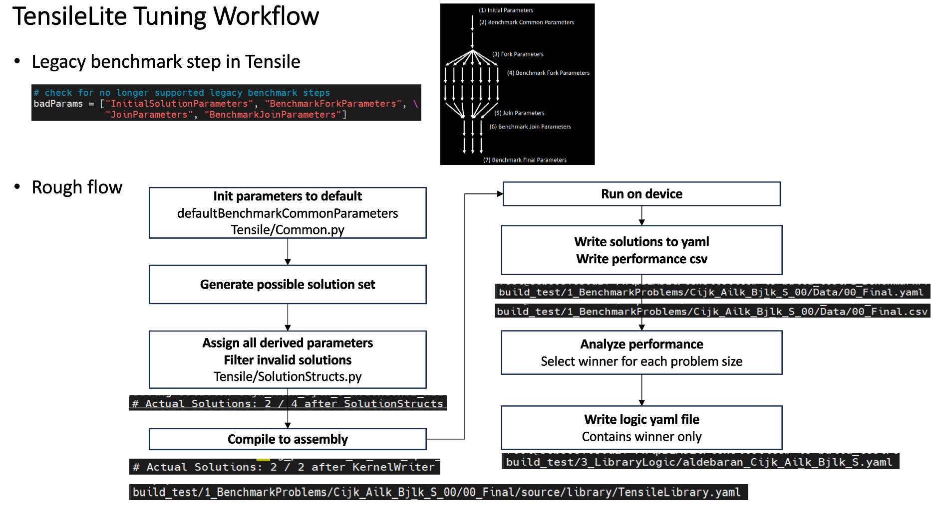
TensileLite tuning flow

Update logic YAML files

The logic YAML files in hipBLASLt are located in library/src/amd_detail/rocblaslt/src/Tensile/Logic/asm_full/.

To merge the YAML files from the tuned results in TensileLite, use the merge.py located in tensilelite/Tensile/Utilities with the following command:

merge.py original_dir new_tuned_yaml_dir output_dir

The following table describes the logic YAML files.

Logic YAML	Description
Equality	Update the equality file when your tuned YAML is an exact tuning.
GridBased	Update the gridbased file when your tuned YAML is a grid-based tuning.
FreeSize	Update the freesize file when your tuned YAML contains confidential sizes, or others. Note that freesize YAML files do not require any problem size.

Tensile optimization and performance tuning

MI16x16 versus MI32x32

MI16x16 outperforms MI32x32 due to its superior power efficiency. The MI16x16 format refers to the v_mfma instruction (such as v_mfma_f32_16x16x16f16). See https://llvm.org/docs/AMDGPU/AMDGPUAsmGFX940.html#vop3p.

Clock differences among XCDs

There can be a clock speed variation of 3% to 10% among different XCDs. Typically, XCD0 has the highest clock speed, while XCD7 has the lowest on MI300X. For optimal efficiency calculations on MI300X, use the XCD with the lowest average clock speed. If the average clock speed of XCD0 is used, target efficiencies (such as, 95% for DGEMM HPL cases with K=512) may not be achievable.

WorkGroupMapping

To maximize L2 cache efficiency, use multiples of the XCD number. For MI300X, this means using multiples of 8 (such as, 24, 32, 40).

GEMM stride issues

On MI300, if the matrix stride in GEMM is a multiple of 512 bytes, it can lead to Tagram channel hotspotting issues, causing a significant performance drop, especially for TN transpose cases. This can increase the latency of VMEM instructions and cause a notable performance drop. To avoid this, use stride padding to ensure the stride is not a multiple of 512 bytes (for instance, for TN F16 GEMM, set lda = ldb = K + 128 when K % 256 == 0).

Optimizing Composable Kernel GEMM kernels

The performance of a GEMM kernel is significantly influenced by the input values. The performance hierarchy based on input value types, from highest to lowest, is as follows:

• Case 1: [all 0]

• Case 2: [all identical integers]

• Case 3: [random integers]

• Case 4: [random floats]

There can be more than a 20 percent performance drop between Case 1 and Case 4, and a 10 percent drop between random integers and random floats.

Additionally, bf16 matrix core execution is noticeably faster than f16.

Distributing workgroups with data sharing on the same XCD can enhance performance (reduce latency) and improve benchmarking stability.

CK provides a rich set of template parameters for generating flexible accelerated computing kernels for difference application scenarios.

See Optimizing with Composable Kernel for an overview of Composable Kernel GEMM kernels, information on tunable parameters, and examples.

MIOpen

MIOpen is AMD’s open-source, deep learning primitives library for GPUs. It implements fusion to optimize for memory bandwidth and GPU launch overheads, providing an auto-tuning infrastructure to overcome the large design space of problem configurations.

Convolution

Many of MIOpen kernels have parameters which affect their performance. Setting these kernel parameters to optimal values for a given convolution problem, allows reaching the best possible throughput. The optimal values of these kernel parameters are saved in PerfDb (Performance database). PerfDb is populated through tuning. To manipulate the tuning level, use the environment variable MIOPEN_FIND_ENFORCE (1-6). Optimal values of kernel parameters are used to benchmark all applicable convolution kernels for the given convolution problem. These values reside in the FindDb. To manipulate how to find the best performing kernel for a given convolution problem, use the environment variable MIOPEN_FIND_MODE (1-5).

Tuning in MIOpen

MIOPEN_FIND_ENFORCE=DB_UPDATE, 2

Performs auto-tuning and update to the PerfDb.

MIOPEN_FIND_ENFORCE=SEARCH, 3

Only perform auto-tuning if PerfDb does not contain optimized value for a given convolution problem

What does PerfDb look like?

[
 2x128x56xNHWCxF, [
                  ConvAsm1x1U          :  1,8,2,64,2,4,1,8 ;       // optimum kernel params for convolution problem 2x128x56xNHWCxF
                  ConvOclDirectFwd1x1  : 1,128,1,1,0,2,32,4,0;     // optimum kernel params for convolution problem 2x128x56xNHWCxF
                  ],
2x992x516xNHWCxF, [
                  ConvAsm1x1U          :  64,18,2,64,2,4,41,6 ;    // optimum kernel params for convolution problem 2x992x516xNHWCxF
                  ConvOclDirectFwd1x1  : 54,128,21,21,1,23,32,4,0  // optimum kernel params for convolution problem 2x992x516xNHWCxF
                  ]
 ...
]

See Using the performance database for more information.

Finding the fastest kernel

MIOPEN_FIND_MODE=NORMAL, 1

Benchmark all the solvers and return a list (front element is the fastest kernel).

MIOPEN_FIND_MODE=FAST, 2

Check FindDb (Find database) if convolution problem is found return - else immediate fallback mode (predict the performing kernel parameters based on mathematical and AI models).

MIOPEN_FIND_MODE=HYBRID, 3

Check FindDb if convolution problem is found return - else benchmark that problem.

What does FindDb look like?

[

 2x128x56xNHWCxF, [
                  ConvAsm1x1U          :  0.045 (time), 12312 (workspace), algo_type;
                  ConvOclDirectFwd1x1  : 1.145 (time), 0 (workspace), algo_type;
                  ],

2x992x516xNHWCxF, [
                  ConvAsm1x1U          :  2.045 (time), 12312 (workspace), algo_type;
                  ConvOclDirectFwd1x1  : 1.145 (time), 0 (workspace), algo_type;
                  ]
 ...
]

See Using the find APIs and immediate mode for more information.

For example:

MIOPEN_FIND_ENFORCE=3 MIOPEN_FIND_MODE=1 ./bin/MIOpenDriver convbfp16 -n 1 -c 1024 -H 14 -W 14 -k 256 -y 1 -x 1 -p 0 -q 0 -u 1 -v 1 -l 1 -j 1 -m conv -g 1 -F 1

RCCL

RCCL is a stand-alone library of standard collective communication routines for GPUs, implementing all-reduce, all-gather, reduce, broadcast, reduce-scatter, gather, scatter, and all-to-all. RCCL supports an arbitrary number of GPUs installed in a single node or multiple nodes and can be used in either single- or multi-process (such as MPI) applications.

The following subtopics include information on RCCL features and optimization strategies:

• Use all eight GPUs

• Disable NUMA auto-balancing

• Disable ACS for multi-node RCCL

• Run RCCL-Unittests

• NPKit profiler

• RCCL-tests

• Use one-process-per-GPU mode

• RCCL in E2E workloads

Use all eight GPUs

In an MI300X architecture, there are dedicated links between each pair of GPUs in a fully connected topology. Therefore, for collective operations, the best performance is achieved when all 8 GPUs and, hence, all the links between them are used. In the case of 2- or 4-GPU collective operations (generally less than 8 GPUs), you can only use a fraction of the potential bandwidth on the node.

The following figure shows an MI300X node-level architecture of a system with AMD EPYC processors in a dual-socket configuration and eight AMD Instinct MI300X accelerators. The MI300X OAMs attach to the host system via PCIe Gen 5 x16 links (yellow lines). The GPUs use seven high-bandwidth, low-latency AMD Infinity Fabric™ links (red lines) to form a fully connected 8-GPU system.

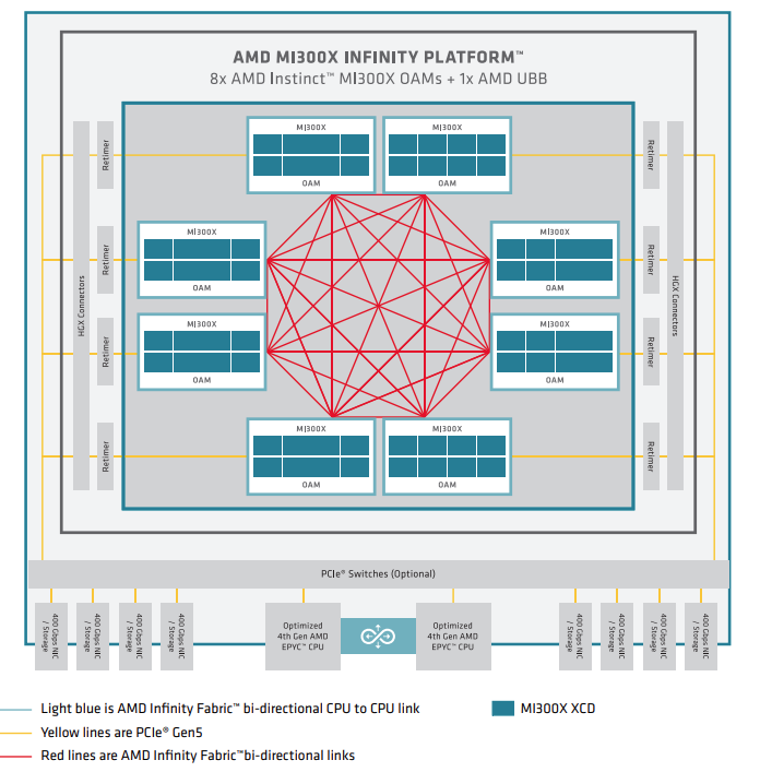
MI300 series node-level architecture showing 8 fully interconnected MI300X OAM modules connected to (optional) PCIe switches via re-timers and HGX connectors.

Disable NUMA auto-balancing

In order to reduce performance variability and also achieve better performance, you need to make sure that NUMA auto-balancing is disabled on the node.

Check whether NUMA auto-balancing is disabled, by running the following command: cat /proc/sys/kernel/numa_balancing and checking whether the output is 0.

If the output is 1, you can disable NUMA auto-balancing by running the following command: sudo sysctl kernel.numa_balancing=0. For more details, see AMD Instinct MI300X system optimization.

Disable ACS for multi-node RCCL

Check if ACS is disabled with sudo lspci -vvv \| grep -i "acsctl". This will print many lines. Check if there are any that show SrcValid+

If there are any SrcValid+, then use the following disable_acs.sh script to disable ACS (requires sudo).

#!/bin/bash

#

# Disable ACS on every device that supports it

#

PLATFORM=$(dmidecode --string system-product-name)

logger "PLATFORM=${PLATFORM}"

# Enforce platform check here.

#case "${PLATFORM}" in

#"OAM"*)

#logger "INFO: Disabling ACS is no longer necessary for ${PLATFORM}"

#exit 0

#;;

#*)

#;;

#esac

# must be root to access extended PCI config space

if [ "$EUID" -ne 0 ]; then

echo "ERROR: $0 must be run as root"

exit 1

fi

for BDF in \`lspci -d "*:*:*" \| awk '{print $1}'`; do

# skip if it doesn't support ACS

setpci -v -s ${BDF} ECAP_ACS+0x6.w > /dev/null 2>&1

if [ $? -ne 0 ]; then

#echo "${BDF} does not support ACS, skipping"

continue

fi

logger "Disabling ACS on \`lspci -s ${BDF}`"

setpci -v -s ${BDF} ECAP_ACS+0x6.w=0000

if [ $? -ne 0 ]; then

logger "Error enabling directTrans ACS on ${BDF}"

continue

fi

NEW_VAL=`setpci -v -s ${BDF} ECAP_ACS+0x6.w \| awk '{print $NF}'\`

if [ "${NEW_VAL}" != "0000" ]; then

logger "Failed to enabling directTrans ACS on ${BDF}"

continue

fi

done

exit 0

Run RCCL-Unittests

In order to verify RCCL installation and test whether all parts and units of RCCL work as expected you can run the RCCL-Unittests which is explained in ROCm/rccl.

NPKit profiler

To collect fine-grained trace events in RCCL components, especially in giant collective GPU kernels you can use the NPKit profiler explained in ROCm/rccl.

RCCL-tests

RCCL-tests are performance and error-checking tests for RCCL maintained in ROCm/rccl-tests.

These tests are one of the best ways to check the performance of different collectives provided by RCCL. You can select collectives, message sizes, datatypes, operations, number of iterations, etc., for your test, and then rccl-tests deliver performance metrics such as latency, algorithm bandwidth, and bus bandwidth for each case.

Use one-process-per-GPU mode

RCCL delivers the best performance for collectives when it is configured in a one-process-per-GPU mode. This is due to the fact that for a one-process-per-multiple-GPUs configuration, you can run into kernel launch latency issues. This is because ROCm serializes kernel launches on multiple GPUs from one process which hurts performance.

RCCL in E2E workloads

Use the following environment variable to increase the number of channels used by RCCL when using RCCL in end-to-end workloads to potentially improve the performance:

export NCCL_MIN_NCHANNELS=112

Triton kernel performance optimization

Triton kernel optimization encompasses a variety of strategies aimed at maximizing the efficiency and performance of GPU computations. These strategies include optimizing overall GPU resource utilization, tuning kernel configurations, and leveraging specific hardware features to achieve higher throughput and lower latency.

Auto-tunable kernel configurations and environment variables

Auto-tunable kernel configuration involves adjusting memory access and computational resources assigned to each compute unit. It encompasses the usage of LDS, register, and task scheduling on a compute unit.

The accelerator or GPU contains global memory, local data share (LDS), and registers. Global memory has high access latency, but is large. LDS access has much lower latency, but is smaller. It is a fast on-CU software-managed memory that can be used to efficiently share data between all work items in a block. Register access is the fastest yet smallest among the three.

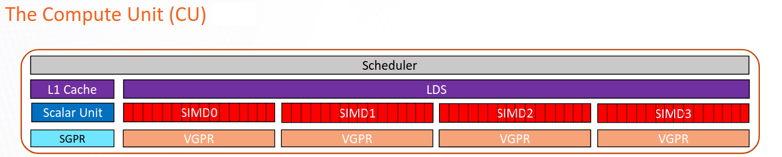
Schematic representation of a CU in the CDNA2 or CDNA3 architecture.

The following is a list of kernel arguments used for tuning performance and resource allocation on AMD accelerators, which helps in optimizing the efficiency and throughput of various computational kernels.

num_stages=n

Adjusts the number of pipeline stages for different types of kernels. On AMD accelerators, set num_stages according to the following rules:

• For kernels with a single GEMM, set to 0.

• For kernels with two GEMMs fused (Flash Attention, or any other kernel that fuses 2 GEMMs), set to 1.

• For kernels that fuse a single GEMM with another non-GEMM operator (for example ReLU activation), set to 0.

• For kernels that have no GEMMs, set to 1.

waves_per_eu=n

Helps to manage Vector General Purpose Registers (VGPR) usage to achieve desired occupancy levels. This argument hints to the compiler to reduce VGPR to achieve n occupancy where n is a number. The goal is to achieve a certain occupancy level for each Execution Unit (EU, also called SIMD Unit) to achieve better latency or throughput. For more information on how to compute occupancy, see Compute the occupancy of a kernel.

This argument is useful if:

• The occupancy of the kernel is limited by VGPR usage, and

• The current VGPR usage is only a few above a boundary in Occupancy related to VGPR usage in an Instinct MI300X accelerator.

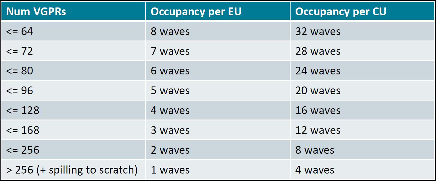
Occupancy related to VGPRs usage on an Instinct MI300X accelerator

For example, according to the table, the available VGPR is 512 per Execution Unit (EU), and VGPU is allocated at the unit of 16. If the current VGPR usage is 170, the actual requested VGPR will be 176, so the occupancy is only 2 waves per EU since \(176 \times 3 > 512\). So, if you set waves_per_eu to 3, the LLVM backend tries to bring VGPR usage down so that it might fit 3 waves per EU.

BLOCK_M, BLOCK_N, BLOCK_K

Tile sizes to be tuned to balance the memory-to-computation ratio. The goal is to minimize the memory transfer from global to shared and reuse memory across different threads. This needs to be tuned. The tile sizes should be large enough to maximize the efficiency of the memory-to-computation ratio but small enough to parallelize the greatest number of workgroups at the grid level.

matrix_instr_nonkdim

Experimental feature for Flash Attention-like kernels that determines the size of the Matrix Fused Multiply-Add (MFMA) instruction used.

• matrix_instr_nonkdim = 16: mfma_16x16 is used.

• matrix_instr_nonkdim = 32: mfma_32x32 is used.

For GEMM kernels on an MI300X accelerator, mfma_16x16 typically outperforms mfma_32x32, even for large tile/GEMM sizes.

The following is an environment variable used for tuning.

OPTIMIZE_EPILOGUE

Setting this variable to 1 can improve performance by removing the convert_layout operation in the epilogue. It should be turned on (set to 1) in most cases. Setting OPTIMIZE_EPILOGUE=1 stores the MFMA instruction results in the MFMA layout directly; this comes at the cost of reduced global store efficiency, but the impact on kernel execution time is usually minimal.

By default (0), the results of MFMA instruction are converted to blocked layout, which leads to global_store with maximum vector length, that is global_store_dwordx4.

This is done implicitly with LDS as the intermediate buffer to achieve data exchange between threads. Padding is used in LDS to avoid bank conflicts. This usually leads to extra LDS usage, which might reduce occupancy.

Note

This variable is not turned on by default because it only works with tt.store but not tt.atomic_add, which is used in split-k and stream-k GEMM kernels. In the future, it might be enabled with tt.atomic_add and turned on by default.

Overall GPU resource utilization

As depicted in the following figure, each XCD in MI300X contains 40 compute units (CUs), with 38 active. Each MI300X contains eight vertical XCDs, and a total of 304 active compute units capable of parallel computation. The first consideration is the number of CUs a kernel can distribute its task across.

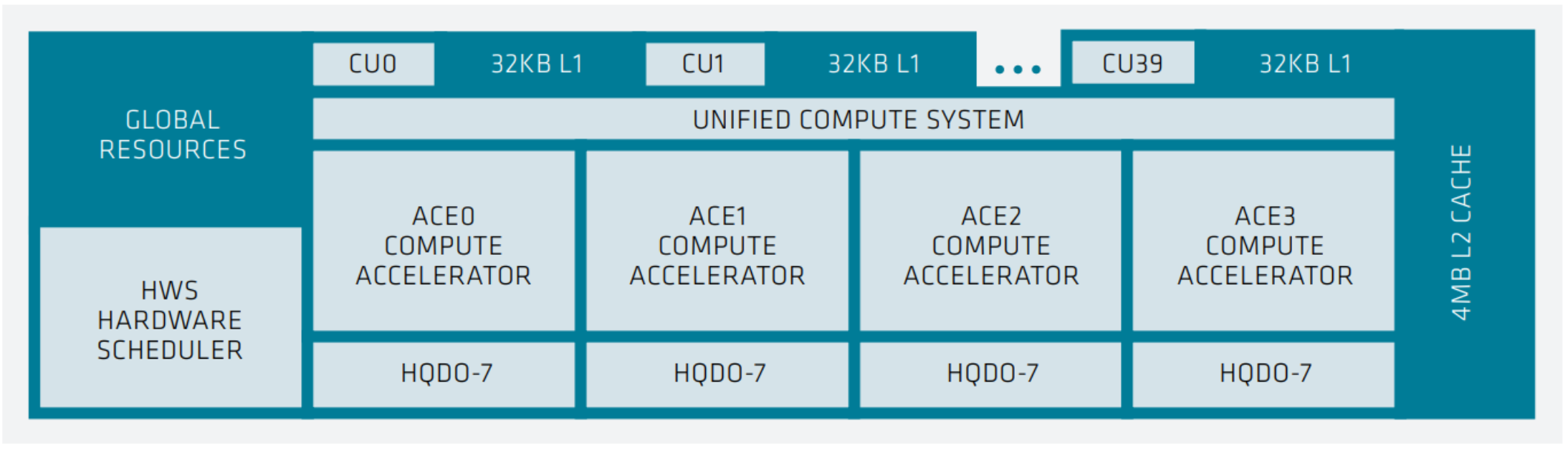
XCD-level system architecture showing 40 compute units, each with 32 KB L1 cache, a unified compute system with 4 ACE compute accelerators, shared 4MB of L2 cache, and a hardware scheduler (HWS).

You can query hardware resources with the command rocminfo in the /opt/rocm/bin directory. For instance, query the number of CUs, number of SIMD, and wavefront size using the following commands.

rocminfo | grep "Compute Unit"

rocminfo | grep "SIMD"

rocminfo | grep "Wavefront Size"

For the MI300X, the goal is to have a minimum of 1024 thread blocks or workgroups in the grid (kernel), with a preference for more.

Identifying additional parallelism within the algorithm is necessary to enhance GPU utilization. For more information and examples, see Accelerating A Triton Fused Kernel For W4a16 Quantized Inference With SplitK Work Decomposition.

MLIR analysis

Triton includes the following layouts: blocked, shared, sliced, and MFMA.

Use the Triton GPU Intermediate Representation (IR) to identify the memory in which each computation takes place.

Use the environment variable MLIR_ENABLE_DUMP to dump MLIR:

export MLIR_ENABLE_DUMP=1

The following is a snippet of IR from the Flash Attention decode int4 KV program. It is to de-quantize the int4 key-value from the int4 data type to fp16.

%190 = tt.load %189 {cache = 1 : i32, evict = 1 : i32, isVolatile =
false} : tensor<1x64xi32, #blocked6> loc(#loc159)

%266 = arith.andi %190, %cst_28 : tensor<1x64xi32, #blocked6>
loc(#loc250)

%267 = arith.trunci %266 : tensor<1x64xi32, #blocked6> to
tensor<1x64xi16, #blocked6> loc(#loc251)

%268 = tt.bitcast %267 : tensor<1x64xi16, #blocked6> -> tensor<1x64xf16,
#blocked6> loc(#loc252)

%269 = triton_gpu.convert_layout %268 : (tensor<1x64xf16, #blocked6>) ->
tensor<1x64xf16, #shared1> loc(#loc252)

%270 = tt.trans %269 : (tensor<1x64xf16, #shared1>) -> tensor<64x1xf16,
#shared2> loc(#loc194)

%276 = triton_gpu.convert_layout %270 : (tensor<64x1xf16, #shared2>) ->
tensor<64x1xf16, #blocked5> loc(#loc254)

%293 = arith.mulf %276, %cst_30 : tensor<64x1xf16, #blocked5>
loc(#loc254)

%295 = arith.mulf %292, %294 : tensor<64x32xf16, #blocked5> loc(#loc264)

%297 = arith.addf %295, %296 : tensor<64x32xf16, #blocked5> loc(#loc255)

%298 = triton_gpu.convert_layout %297 : (tensor<64x32xf16, #blocked5>)
-> tensor<64x32xf16, #shared1> loc(#loc255)

%299 = tt.trans %298 : (tensor<64x32xf16, #shared1>) ->
tensor<32x64xf16, #shared2> loc(#loc196)

%300 = triton_gpu.convert_layout %299 : (tensor<32x64xf16, #shared2>) ->
tensor<32x64xf16, #triton_gpu.dot_op<{opIdx = 1, parent = #mfma, kWidth
= 4}>> loc(#loc197)

From the IR snippet, you can see i32 data is loaded from global memory to registers (%190). With a few element-wise operations in registers, it is stored in shared memory (%269) for the transpose operation (%270), which needs data movement across different threads. With the transpose done, it is loaded from LDS to register again (%276), and with a few more element-wise operations, it is stored to LDS again (%298). The last step loads from LDS to registers and converts to the dot-operand layout (%300).

The IR snippet uses the LDS twice. The first is for the transpose, and the second is to convert a blocked layout to a dot operand layout. There’s an opportunity to optimize performance by using LDS once.

ISA assembly analysis

To generate ISA, export AMDGCN_ENABLE_DUMP=1 when running the Triton program. The generated ISA will be printed as standard output. You can dump it to a file for analysis.

• Ensure global_load_dwordx4 is used in the ISA, especially when the global memory load happens in the loop.

• In most cases, the LDS load and store should use _b128 to minimize the number of LDS access instructions.

• The AMD ISA has s_waitcnt instruction to synchronize the dependency of memory access and computations. The s_waitcnt instructions can typically have two signals in the Triton context:

  • lgkmcnt(n): lgkm stands for LDS, GDS (Global Data Share), Constant, and Message. It is often related to LDS access. The n indicates the number of data accesses can still be ongoing before moving on to the next step. For example, if n is 0, wait for all lgkm access to finish before continuing. If n is 1, move on even if 1 lgkm access is still running asynchronously.

  • vmcnt(n): vm represents vector memory. This happens when vector memory is accessed, for example, when global load moves from global memory to vector memory. The variable n is the same as the previous setting.

Generally recommended guidelines are as follows.

• Vectorize memory access as much as possible.

• Ensure synchronization is done efficiently.

• Overlap of instructions to hide latency, but it requires thoughtful analysis of the algorithms.

• If you find inefficiencies, you can trace it back to LLVM IR, TTGIR and even TTIR to see where the problem comes from. If you find it during compiler optimization, activate the MLIR dump (export MLIR_ENABLE_DUMP=1) and check which optimization pass caused the problem.

HIP performance optimization

This section summarizes the best practices described in the Performance guidelines section of the HIP documentation.

Optimization areas of concern include:

• Parallel execution

• Memory usage optimization

• Optimization for maximum throughput

• Minimizing memory thrashing

Parallel execution and GPU hardware utilization

The application should reveal and efficiently imply as much parallelism as possible for optimal use to keep all system components active.

Memory usage optimization

To optimize memory throughput, minimize low-bandwidth data transfers, particularly between the host and device. Maximize on-chip memory, including shared memory and caches, to reduce data transfers between global memory and the device.

In a GPU, global memory has high latency but a large size, while local data share (LDS) has lower latency but a smaller size, and registers have the fastest but smallest access. Aim to limit load/store operations in global memory. If multiple threads in a block need the same data, transfer it from global memory to LDS for efficient access.

See HIP’s performance guidelines for greater detail.

Diagnostic and performance analysis

Debug memory access faults

Identifying a faulting kernel is often enough to triage a memory access fault. The ROCr Debug Agent can trap a memory access fault and provide a dump of all active wavefronts that caused the error, as well as the name of the kernel. For more information, see ROCr Debug Agent documentation.

To summarize, the key points include:

1. Compiling with -ggdb -O0 is recommended but not required.

2. HSA_TOOLS_LIB=/opt/rocm/lib/librocm-debug-agent.so.2 HSA_ENABLE_DEBUG=1 ./my_program

When the debug agent traps the fault, it produces verbose output of all wavefront registers and memory content. Importantly, it also prints something similar to the following:

Disassembly for function vector_add_assert_trap(int*, int*, int*):

code object:
file:////rocm-debug-agent/build/test/rocm-debug-agent-test#offset=14309&size=31336

loaded at: [0x7fd4f100c000-0x7fd4f100e070]

The kernel name and the code object file should be listed. In the example above, the kernel name is vector_add_assert_trap, but this might also look like:

Disassembly for function memory:///path/to/codeobject#offset=1234&size=567:

In this case, it’s an in-memory kernel that was generated at runtime. Using the environment variable ROCM_DEBUG_AGENT_OPTIONS="--all --save-code-objects" will have the debug agent save all code objects to the current directory. Use --save-code-objects=[DIR] to save them in another location.

The code objects will be renamed from the URI format with special characters replaced by ‘_’. Use llvm-objdump to disassemble the indicated in-memory code object that has been saved to disk. The name of the kernel is often found in the disassembled code object.

llvm-objdump --disassemble-all path/to/code-object.co

Disabling memory caching strategies within the ROCm stack and PyTorch is recommended, where possible. This gives the debug agent the best chance of finding the memory fault where it originates. Otherwise, it could be masked by writing past the end of a cached block within a larger allocation.

PYTORCH_NO_HIP_MEMORY_CACHING=1

HSA_DISABLE_FRAGMENT_ALLOCATOR=1

Compute the occupancy of a kernel

1. Get the VGPR count, search for .vgpr_count in the ISA (for example, N).

2. Get the allocated LDS following the steps (for example, L for the kernel).

   1. export MLIR_ENABLE_DUMP=1

   2. rm -rf ~/.triton/cache

   3. python kernel.py | | grep "triton_gpu.shared = " | tail -n 1

   4. You should see something like triton_gpu.shared = 65536, indicating 65536 bytes of LDS are allocated for the kernel.

3. Get number of waves per workgroup using the following steps (for example, nW).

   1. export MLIR_ENABLE_DUMP=1

   2. rm -rf ~/.triton/cache

   3. python kernel.py | | grep "triton_gpu.num-warps " | tail -n 1

   4. You should see something like “triton_gpu.num-warps" = 8, indicating 8 waves per workgroup.

4. Compute occupancy limited by VGPR based on N according to the preceding table. For example, waves per EU as occ_vgpr.

5. Compute occupancy limited by LDS based on L by: occ_lds = floor(65536 / L).

6. Then the occupancy is occ = min(floor(occ_vgpr * 4 / nW), occ_lds) * nW / 4

   1. occ_vgpr \* 4 gives the total number of waves on all 4 execution units (SIMDs) per CU.

   2. floor(occ_vgpr * 4 / nW) gives the occupancy of workgroups per CU regrading VGPR usage.

   3. The true occ is the minimum of the two.

Find the full occ.sh at ROCm/triton.

Special considerations

Multi-GPU communications

Because of the characteristics of MI300X inter-GPU communication and limitation of bandwidth between/among 2 GPUs and 4 GPUs, avoid running workloads that use 2 or 4 GPU collectives. It’s optimal to either use a single GPU (where no collective is required) or employ 8 GPU collectives.

Multi-node FSDP and RCCL settings

When using PyTorch’s FSDP (Full Sharded Data Parallel) feature, the HIP streams used by RCCL and HIP streams used for compute kernels do not always overlap well. To work around the issue, it is recommended to use high-priority HIP streams with RCCL.

The easiest way to do that is to ensure you’re using the nightly PyTorch wheels because this PR didn’t make it into release 2.3 but is part of nightly wheels.

• Set environment variable TORCH_NCCL_HIGH_PRIORITY=1 to force all RCCL streams to be high-priority.

• Set environment variable GPU_MAX_HW_QUEUES=2 from HIP runtime library.

The hardware is most efficient when using 4 HIP streams (or less), and these two environment variables force a maximum of two streams for compute and two streams for RCCL. Otherwise, RCCL is often already tuned for the specific MI300 systems in production based on querying the node topology internally during startup.